One would expect—in any research setting—to find that issues with regard to the field’s findings are shared by all sides of different opinions. This is not the case when it comes to the Race-IQ debate. It has been very clear that while one side (the ‘hereditarians’) is constantly seeking to do more research and settle debates professionally, the other side (the ‘environmentalists’) wants to get stuck on hypothetical quibbles and already settled research. This will be demonstrated below too, and is, in fact, the point of this entire post. I am responding to a bunch of supposed truisms supported by ‘DSTSquad’, and I am planning to make this response a quote by quote one. Because of this, the format may look messy, so, a warning (also a note to whoever is writing the blogposts in that website, stop putting periods next to “et” when citing a paper with ‘et al’, et is not an abbreviation; the period goes after “al” 🙂, you’re welcome).
Heritability is a concept that has been understood for thousands of years, but which has made significant quantitative progress in modern times. It’s very simple to understand. However, it seems some people simply don’t want to understand it, and in turn confuse themselves along with other people, resulting in a complete misunderstanding of what it is. Let’s see a demonstration.
it has long been known that traits that are known to be “genetic” can have heritabilities of 0 (see: the presence of eyes) and traits that are known to be “environmental” can have heritabilities of 1 (see: wearing earrings)
This is obviously true... right? Well, not exactly. Notice how in the first example (which is true), this is something that is easily identifiable because it is way behind in analogical use. Think for just a moment about what heritability is! It is a variance metric. So what does that tell us? It tells us that no variation in something results in what we would call an error in this context: the number 0. This is easily deductible and doesn’t need to be addressed in a complex manner (or any way that takes up more than 5 minutes). Now picture this: instead of measuring the variation with regards to having eyes, let’s measure the variation with regards to eye width. Oh boy, suddenly the heritability isn’t 0. And this is exactly the case with the Race-IQ debate. Everyone has intelligence, so measuring the heritability of that would also be 0. However, measuring the heritability of your intelligence level... that’s a whole different thing. So this can be dismissed entirely. As for the latter part (earrings), that’s just a plain lie, no idea where it came from, so it will be ignored like it deserves to.
if individuals differences in traits (IQ) are ‘attributable’ (purely in a statistical sense) to genes and racial groups differ in traits (IQ), then isn’t it reasonable to conclude that the gap between racial groups in these traits is partially genetic? This is a fallacy that Lewontin identified decades ago by positing a thought experiment
Yes, of course, what is a heritability article without Lewontin’s seed metaphor? First, what exactly is Lewontin’s seed experiment? It’s described here, right next to the latter sentence I quoted:
Suppose we have two plots growing corn. We have a genetically variable set of seeds (all of the same strain) and randomly assign them to each plot. In the first plot we have a uniform environment consisting of high lighting, fertilizer and water, while in the second we have a uniform environment consisting of the absence of lighting, fertilizer and water. Because the environments are uniform in each plot, the heritability of the height of the corn in each plot is respectively, h2 = 1, but the genetic difference in the height between the plots is exactly 0.
OK, so we have another hypothetical in our hands. What can I say… this is pretty convincing. After all, this is true. Yes indeed, this is true, but only theoretically. See, this is actually testable in many ways. This metaphor was something even Galton responded to. It can be handled by assessing the magnitudes of environmental differences, showing the generalizability of g-loadings, heritabilities, and other variables, with recourse to the arguments for/against X-factors (including regression to the mean, SEM, matrix decomposition, etc.), adoption studies, changes in environmental quality failing to associate with changes in racial gaps, or explicit model-fitting for a trait. Woah, I accidentally laid out a bunch of nerd terms here! We’ll get to these when time comes. For now, let’s quote Lubke et al. (2003) on the matter:
Consider a variation of the widely cited thought experiment provided by Lewontin (1974), in which between-group differences are in fact due to entirely different factors than individual differences within a group. The experiment is set up as follows. Seeds that vary with respect to the genetic make-up responsible for plant growth are randomly divided into two parts. Hence, there are no mean differences with respect to the genetic quality between the two parts, but there are individual differences within each part. One part is then sown in soil of high quality, whereas the other seeds are grown under poor conditions. Differences in growth are measured with variables such as height, weight, etc. Differences between groups in these variables are due to soil quality, while within-group differences are due to differences in genes. If an MI model were fitted to data from such an experiment, it would be very likely rejected for the following reason. Consider between-group differences first. The outcome variables (e.g., height and weight of the plants, etc.) are related in a specific way to the soil quality, which causes the mean differences between the two parts. Say that soil quality is especially important for the height of the plant. In the model, this would correspond to a high factor loading. Now consider the within-group differences. The relation of the same outcome variables to an underlying genetic factor are very likely to be different. For instance, the genetic variation within each of the two parts may be especially pronounced with respect to weight-related genes, causing weight to be the observed variable that is most strongly related to the underlying factor. The point is that a soil quality factor would have different factor loadings than a genetic factor, which means that the undergirding equations cannot hold simultaneously. The MI model would be rejected.
So, yes, Lewontin made a hypothetical which is true, as in, it syllogistically makes sense. If only it were also practically true… since it isn’t, and we know it isn’t because of, well for one, Turkheimer, which showed us in one of his later published theses that it is a mathematical necessity that within and between-group variance components relate to one another; they cannot be independent without extremely strong X-factors which are systematic with respect to each of any group (though contained within a measured variance component). In fact, we can determine how large the (supposedly fully-causal) environmental difference (X) must be as a matter of simple algebra since:
\(X = \frac{d}{\sqrt{1-h^2}}\)
where X = the environmental difference, d = the size of the group difference, and √(1 - h²) being Jensen’s 1998 formula applied to our variables. So, if we go with the existing between-group racial difference in psychometric g (over 1 SD) and the (lowballed) Wilson effect heritability of 0.8, we get that the environment of the average black person must be 2.46 d worse than the average white environment (~99% of whites will have better environments than blacks, which is obviously absurd). Since the only variance components remaining in adulthood are A and E (again, see Wilson effect), this worse environment must be somehow systematic with respect to race and unsystematic with respect to siblings (hint: this is impossible). On the other hand, if we do allow some shared environmental variance to exist, then the formula becomes:
\(X = \sqrt{d-(1-A^2)}\sqrt{C^2}\)
Which still requires unfathomably large environmental differences.
Now that we know that Lewontin’s seed metaphor isn’t real, we can throw it out the window as another theoretical attempt (they keep piling up). Moving on.
the question of whether ‘nature’ or ‘nurture’ contributes more is a question that fundamentally doesn’t make sense. As an analogy, suppose Jack and Jill are filling up a bucket together. Jill brought the bucket to their spot and Jack brought the hose. They fill up the bucket together. The question “how much of the water is attributable to Jack vs Jill” is not just the wrong question, but altogether absurd!
So now we’ve reached the point beyond the façade, where this person outright claims they believe heritability is not even a variance metric. This obvious tautological error aside, the question actually does make sense. Let’s use our brains for more than 10 seconds. We are all familiar with ACE/ACDE models of heritability (I assume, if you aren’t, go read about them here). Well, how do they relate? We know they encapsulate specific variance components, but these are important on the theoretical level here. What exactly would Jack’s contribution be in this analogy? Well, it would fall under the D component, or in other words, non-additive/broad/indirect genetic effects. Why? Well, because Jack isn’t directly pouring water into the bucket, he is indirectly doing it by opening the tap, whereas Jill would be the A component (additive genetic effects) since she is directly responsible for pouring the water into the bucket. So, we would actually be able to measure how much of the water filled was due to Jack or Jill, given we encapsulate what we mean by “broad-sense” and “narrow-sense” well.
What’s important to note here is that there a number of assumptions in these calculations. First, as we noted above, is the assumption that MZ twins share the same level of environmental similarity as DZ twins, which we have good reason to believe is false
Now we move on to assumptions. Hot! Notice how the paper they cite is about schizophrenia. This is an important detail because this assumption of environmental similarity is only important when it comes to trait-relevant environments! Guess what, there is no such variance in environments in reared-together twins (from here). Can we test for reared-apart twins? Yes, adoption studies (transracial, even), not much difference at all. So no, we do not have any reason to believe the EEA is false. But, we’ll also get to that later.
Second is the absence of gene-environment interaction
Other assumption violations include the presence of gene-environment correlation, dominance (in the presence of which estimates based on MZ and DZ twins are upwardly biased), epistasis and associative mating
Ignoring that these are not assumption violations, they are also testable. So what do we have on them?
You cannot ignore gene-environment correlations if you want to talk about GxE. That’s silly. And for the rest you can read the papers (underestimates, again). That’s about it.
The most robust estimates I’ve seen that take into account all family data (parent-child, twin, adoptee, etc correlations) to produce a single set of estimates
They cite Cloninger et al. (1979a, 1979b); Rice et al. (1978); Rao et al. (1982); Chipuer et al. (1990); Devlin et al. (1997), and Devlin, Daniels and Roeder (1997). Wow. Impressive amount of papers here. Now if one actually reads them, they notice very quickly that this is just a gish-gallop. These papers are virtually the same. No adult samples (Wilson effect), no real data (baseless beliefs of attenuation with no empirical testing of whether this is in fact the case, just modelling what effects could be), they assume certain variance components don’t fadeout into adulthood (they do), their original datasets find heritabilities very well over 70% (see, e.g., Bouchard & McGue, 1981). They also cite Otto, Christiansen, and Feldman (1995), though thankfully we now know that cultural effects have g-loadings of ~-1 (and we have measurement invariance), so this is irrelevant. Though in this attempt to gish-gallop, they also slip in the largest twin meta ever, Polderman et al. (2015)! Guess what they found (not mentioning an entire section dedicated to explaining their estimates are deflated):
Wilson effect vindicated again (never-mind the decline in ages >65)! Oh boy... and what about the MZ-DZ correlations? They seem spurious, one might say. Well, go to ‘Effect vs. Sample Size‘ and you will eyeball the margin of error. No biggie though, they cite it with no regrets!
Starting strong! Unrelated to the Wilson effect entirely... but let’s address them too, independently of the criticisms of the article. First, the Rothstein paper is the Sociologist’s Fallacy at work. They ‘adjust for income’ (presumably for no reason other than to close the gap artificially), which is problematic as it’s a baseless control and doesn’t even make sense, given that higher IQ individuals earn higher income, so going up in income brackets will also obviously go up in IQ ones, just not for reasons of IQ interventions (rather, the exact opposite). As for the Rindermann analyses, they’re a bit sketchy. For Rindermann & Thompson, I’m not certain that there was a large narrowing in the magnitude of the B/W achievement gap. When looking at all of the NAEP MAIN assessments, you can find a d-value of ~ 0.95, and a d-value of ~1.0 when looking at the most recent PISA and TIMSS results:
There’s something odd going on here. Can’t say for sure, but teaching the tests seems likely. Rindermann and Thompson (2013) also offer many hypotheses on why IQ advances for older youths may have plateaued. The long-term advantages may simply have accelerated child growth. Alternatively, the genetic influences get stronger from infancy to maturity, or that the impact of preschool changes is diminishing, or that, today, there is more negative peer pressure in adolescence against learning than ever before, or perhaps that secondary school instructional quality improves (or deteriorates) less than primary school instruction, and so on. Yes, early-life gains do not always translate to later-life gains, and Grissmer et al. (1998) find this trend consistent with the broader notion that education programs do not raise IQ in the long term. However, Grissmer also discusses the idea of changing the difference at later years while keeping the gap at younger ages constant through time. For example, whereas the high school curriculum may have become more difficult over time, the elementary school curriculum remained unaltered. Accordingly, the authors are essentially arguing that curriculum should have been made very demanding at both an earlier and later age if measures to raise IQ at maturity had failed. But there’s an issue: IQ is not this. Jensen (1973) defined intelligence as “the ability to understand the material that has been taught”. If cognitive abilities require perseverance in rehearsing of acquired knowledge in order to be sustained, the gains cannot be g-loaded. They got it all wrong before adding controls and making their code. Similarly, Rindermann & Pichelmann are also weird. Not only do they find the exact same results under the exact same assumptions, they happen to report their effect sizes on table 8, and... well... one could say this wasn’t a very good idea.
All of their effect sizes are below the “small” range (except one in eminor which is .1 above small). But notice this: They are small until the prediction model comes in. That is, whilst their findings have tiny effect sizes, the predictions made from these findings have large ones. That is most certainly odd. These papers aren’t very good evidence as we don’t have access to the tests, and they seem very sketchy to say the least. Besides, they are the only two findings in the literature supporting this finding (aside from the Dickens & Flynn cases which only show closings in the Stanford-Binet and children samples). Another comprehensive meta-analysis found no closing in 150 years tested in all of these datasets. But moving on from this.
more robust and comprehensive reviews of the literature show the effect is non-linear and that the shared environment component may not reach zero in adulthood (Dickens & Protzko 2015)
More robust, presumably for no reason. It doesn’t matter whether C goes to exactly 0 in adulthood. The Dickens paper finds a C of ~.15 in adulthood. Largely irrelevant, you could even say that finding 20% means nothing as the Wilson effect finds heritabilities of close to 80%, so that remaining 20% could be all that there is. Further, the Dickens paper says:
We can find no evidence that shared-environment explains any variance of cognitive ability in adults within races or ethnic groups.
So, wow. Moving on though.
That this heritability coefficient increases over time does not mean something becomes ‘more genetic’ and/or ‘less environmental’
Actually, it may. We know that genes tend to express themselves less/more as age increases for many traits. This also explains – along with the increase in heritability due to the Wilson effect – the decrease in heritability in people over 65 years old.
heritability coefficients only have interpretations for a given population, in a given environment, at a given time
Do they? This is testable. Scarr-Rowe effects are supposed to encapsulate all three of these components. So, what do they show us? Take a look:
So, no differences, and if anything there is an upwards bias for the black sample, i.e., heritability in black people is slightly higher than in whites. So that is also wrong.
A change in the heritability statistic can reflect any of those factors, or others
It cannot. By design, ACDE models encapsulate the vast majority of variance in these components, A = additive genetic influences, C = shared environmental influences, D = indirect genetic influences, E = unique environmental influences, and then we have Assortative Mating, Violations of The EEA, and Measurement Error. That’s about it. Any other factors will be so minute, they will practically inevitably reflect less than 1% of the variance.
not a single gene that is purportedly “for” intelligence has been shown to differentially express itself by age to demonstrate the coherence of the Wilson effect
What a silly claim to make. We’ve never tested for this, so obviously no gene has been shown to do this.
Moreover, there is a question of whether IQ scores are measurement invariant across age cohorts and are commensurable as such, which has been shown to be violated in some samples (Wicherts et. al 2004, Hertzog & Bleckley 2001)
There is no question. Here only Wicherts did not find invariance tenable across age, but the only reason is because of the Flynn effect.
Niileksela obviously did not find invariance since their sample consisted of 70 year olds that only took some previously missing subtests. Bowden found invariance across age cohorts tenable (“Overall, the evidence pointed to invariance across age of a modified 4-factor model that included cross-loadings for the Similarities and Arithmetic subtests”). Multiple other studies report invariance across age groups (e.g., Schaie et al., 1998; Horn & McArdle, 1992; Sprague et al., 2017, etc.). So, we have one study that did not find invariance across age for methodological reasons, and at least 4 that did. Definitely 0 question here.
Despite the so-called “evidence” Bouchard marshals in support of the Wilson Artefact, there is a growing literature (and actually historical!) showing that the assumptions behind the methodology used to “observe” the Wilson effect are violated.
Not quite, and just this year we got another paper vindicating it through showing heritability declines, same way Niileksela et al. (2013) did. This is entirely expected for 60-70 year olds. But we’ll get to that just now.
The first paper published in this vein comes all the way from the 1930s; Wright (1931) fit a path analysis model to Burks IQ data and estimated that the heritability of IQ in childhood is .50, while it is .30 in adulthood
Awesome. We start off with just plain lies. There is no such figure in the paper (except the 50% which is only for Burk’s uncorrected data & is described as being ‘in at least qualitative agreement’ with 0.75). Though, in Wright’s third chart we see that the standardized weight of heredity on child’s IQ is 0.90 for non-adopted children and .96 for adopted ones:
Let’s take the smaller value, 0.90. What does squaring that give us? .81, which is the h2 value. And don’t just take my word for it: Feldman & Ramachandran (2018) get a value of .75 from wright’s analysis with additional controls. So the heritability is actually shown to be 75-81%, not 30, wherever that came from.
Rao et. al (1976) fit large corpuses of IQ data to path analysis models in adulthood and childhood and found that the heritability of intelligence is smaller in adulthood than in childhood
Not sure where this is found. Though in table 8 they find that the heritability without “controlling for” GxE ranges from .41 to .73.
Rao et. al (1982) found that the heritability of IQ increased in adulthood for phenotypic homogamy, and decreases in adulthood for social homogamy (social homogamy seems to be the case for IQ, Keller et. al (2019))
Assortative Mating results from both, not just social homogamy. Keller et al. doesn’t make this case either. Not very conclusive evidence even if they did considering the small association.
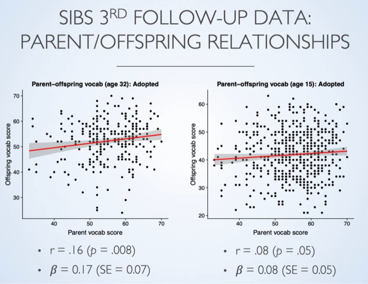
A very recent adoption study has actually observed increasing correlations of adoptive parents to adopted children over time, meaning an increasing effect of shared environment over time
No. Again, this is just lying.
Correlation increases for IQ subtests, not shared environmental variance. This paper also supports a Wilson effect.
A later study, Devlin et. al (1997) used Bayesian inference to test age-effects models against their maternal effects model and found that all age-effects models were inferior (in terms of the Bayes factor).
This is true, but kind of irrelevant. Besides McGue (1997) mentioning how age may have biased heritability downwards in such a model, the authors attribute MZ twin similarity in excess of their heritability estimate (0.48) to shared prenatal environmental effects. This is a problem because it is 1) an assumption, and 2) against most data. Much work shows prenatal effects as important as sharing a chorion are tiny for IQ differences or covariances. Other factors such as foetal position, order of delivery, and blood tranfusion (including ITTS, also there is overlap between study factors) actually appear to differentiate MZ twins rather than increase their similarity (for this see also Loos et al., 2001; Marceau et al., 2016).
Third is another explanation for the “Wilson effect”, namely that of test construction.
And here we have some Race__Realist crankery. Should show you this person’s credibility. Now, yes, what RR is saying in that Twitter thread could be true if… the decline between IQ and heritability was synonymous. Not only are they two different things, the source he cites mentions that the IQ decline begins at 18, whereas we know from the Wilson effect that heritability declines at ages typically over 60 (two things he conflates). How could this possibly be the case? We’ll get to this below.
Thought this was worth adding here since the source material is good, but this is irrelevant to the discussion.
nor is there a theory of “intelligence” (Richardson 2002, 2017) that one can verify “increasing heritability of IQ” with
Again, largely irrelevant source, but this is wrong. There is a theory, it’s called g-theory. Besides the explanation of gene expression (mapping onto g if it is highly heritable), we could see what the increase/decline in heritability is due to. We have this neat metric called the “variance explained”. Even not using that, it’s a basic observation: do g-loadings change with age? If they do, then the heritability change is due to g. If they do not, it’s not due to g. Though, this isn’t even it! The evidence shows that the importance of g does not increase with age. So, the heritability increase seems to be due to non-genuine ability changes (i.e. score variance, not actual abilities). There you go, it’s explained.
And finally, there are gene-environment interaction and gene-environment (evocative and active) correlation explanations of the increase. For example, it could be that small (heritable) differences in IQ at the beginning of development are magnified through processes of niche construction and environmental choice, inducing gene-environment correlations that bias heritability estimates
For this to be the case, you would have to assume GxE does not bias systematically throughout age. It most likely does, so this should be wrong, since we would expect heritability biases from GxE to explain the same amount of variance in childhood and adulthood. Overall not very convincing.
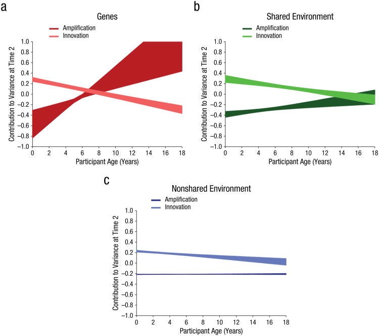
These studies do no such thing. They are developmental models trying to explain the Flynn effect and IQ changes, unrelated to the Wilson effect with regards to GxE. Though, the Briley meta-analysis is related. What does it show?
In the very early years of life, innovative genetic influences appear to account for the increase in heritability. By approximately age 8, genetic amplification effects become predominant and innovative genetic effects reach zero. However, the primary model did not estimate the genetic amplification parameter very precisely, as is evident by the wide shading, rendering interpretation somewhat difficult. The alternative models imply a more gradual slope but with much greater precision.
In short, it’s genetics. The misrepresentation of papers is starting to get kind of weird, no offense. It’s also weird how in a post attempting to disprove the Wilson effect by citing studies finding declines in heritability, there also exist citations proving the Wilson effect multiple times (e.g., again, this very meta).
Other developmental explanations include the accumulation of the violation of the EEA over time, in addition to the unique sociocognitive effects of dizygotic twin relationships (Richardson & Norgate 2005)
Well, we’ve already been through the latter part. So what about the Equal Environmental Assumption? Does it explain the increase in heritability? No (because of this result of twins being misidentified by zygosity being negative and all-else being small). Boring answer, but that’s it. As for Richardson & Norgate (two individuals historically misrepresenting evidence in the literature), it’s basically the same argument Joseph (1998) proposes, which states that MZ similarity is more than DZ similarity, though ignores that this should only be relevant with regards to trait-relevant environments. This is seen in Richardson & Norgate’s paper:
It is known that numerous aspects of home and other experience are much more similar for MZ twins than for DZ twins.
A little after, they propose GxE effects may invalidate the EEA, and try to disprove evidence by handwaving it away as unrepresentative to cognitive abilities. Of course, we’ve already been through these effects and some of the papers (and you’ll notice this trend a lot while reading, mainly because the people writing these pieces are running out of explanations), so we can safely move on.
Such a differential association could also be the result of emergent developmental processes
Interesting. Mutualists tried to explain the increase in the heritability of g, but ultimately failed as, quote:
As a formal model, the mutualism model describes intraindividual change (growth) in a given cognitive ability as a function of both (1) autonomous growth, i.e., growth that does not dependent upon other cognitive abilities, and (2) growth due to the influence of the development of other cognitive abilities.
But... let’s not forget the response. I’m kidding. Forget about it since everything that’s stated there is responded to here (except that age-related SNP part, but nobody cares about that really).
(Dis)Assortative Mating?
Disassortative mating is a real thing in genetics, however people choose to ignore it in favor of assortative mating, because the latter is shown to bias heritabilities. But are they biased downwards or upwards? This post argues an inflation. Let’s review.
Although a little bad-faith, the post provides plenty of supposed evidence to this effect. Starting, we get this:
When confronted with evidence from statistical genetics that heritability estimates from kinship studies have been overestimated (Young et. al 2018, Kemper et. al 2021), typically hereditarians resort to either claiming that the results from statistical genetics are “implausible” and reject them based on the preconceived notion that certain traits have particular heritabilities 1 or claim that there is downward bias in genetic estimates of heritability.
Woah, twin heritability estimates are overestimated? How can this be?! Well let’s examine the citations. First off, Kemper et al. can go away as it validates twin narrow-sense heritabilities (since their model does not include non-additivity; no idea why it was cited here... ahem). But what about Young’s method? His models can include non-additive variance, no? Yes, they can, however there are some assumptions that are not empirically borne out. We will go through them later.
The first is estimates of heritability from genome-wide association studies (GWAS)
I will not discuss GWAS at-length here since that has been done to death already. The TL;DR is that they are kind of underpowered. Yes, like DSTS says, there is no bias due to sample size, but power difficulties remain. What’s more, GWAS typically analyze genetic variants individually and do not capture interactions between multiple genes or variants. Complex traits (like intelligence) involve interactions between multiple genes, i.e. epistasis (& on another note, dominance), and these interactions can be challenging to detect. GWAS also miss the contribution of rare variants (despite these not entirely explaining the missing heritability like DSTS points out), and smaller ones even if common. They’re just not very good for now.
The second line of evidence is that of relatedness disequilibrium regression (RDR) (Young et. al 2018) […] RDR basically extends twin studies by expanding the moments of genetic similarity to very distantly related individuals to estimate the value of heritability without environmental bias
Now onto the issues. To get straight to the point, the method hinges on the assumption that environmental effect bias heritability estimates whenever that might not be the case. A few examples of them being violated include the fact that MZ twins reared-apart give similar heritability estimates (1, 2); unrelated individuals reared together prove trivial effects of shared-environment; GREML controls Young attempts to make don’t actually create substantial differences like they do in his model, and so on. More specifically, another assumption is seen in the given covariance model:
where [R_ij] is the relatedness of individual i and individual j; [R_par]_ij is the relatedness of i‘s parents and the parents of j; and [R_o,_par]_ij is the relatedness of i and the parents of j. It is noted that “generally, cov(ϵ) is not known and may resemble R”. Under this model, environmental effects are assumed to be independent across individuals (i.e., that the environment of one individual doesn’t directly affect the environment of another). This is not borne out by the data. In fact the complete opposite is known, given the countless research on peer effects, genetic nurture &c. The model also assumes that environmental effects are random and not systematically related to genetic relatedness (again see Kong et al. 2018).
Long story short, RDR assumes the existence of certain variance components that are either unproven or disproven. It is more assumption-laden and less grounded. This method also can’t offer results different results compared to sibling regressions, and these methods aren’t intended to offer full heritabilities (like twin studies do) anyway. I will not be going through the rest of the article as it’s an attempt to show that modeling AM into RDR does not substantially change heritabilities, which I do not care very much about given the entire point of the article was just shown to be a straw-man (iirc AM is the ‘last refuge’).
EEA: Extensively Employed Assumption?
The Equal Environmental Assumption has long been known to be untrue. Indeed, while it is literally untrue, it is practically true, as has been mentioned in this post already (since it’s only about trait-relevant environments). Will this attempted refutation of it show anything new (spoiler: no).
Most recent is Conley et. al (2013), which purported to find that the equal environment assumption was supported. A closer look at the data supports the opposite conclusion, which I detailed in this thread.
Ah! A paper I cited. Unfortunately their account got suspended, therefore there is no possible way to know what they meant exactly (nothing in archive-sites either). I was really curious, too, since there is absolutely no way I can think of to interpret that data differently. Moving on disappointed.
Now for the sections ‘Environmental Similarity Studies’ and ‘Physical Similarity Studies’, they do not cite any specific cases, so again, nothing to really say, except that I agree with the latter section, though it’s largely irrelevant to this debate since the studies operating under the physical similarity hypothesis are mostly theoretical (as they state most of the time).
Zaitlen et. al (2014) used the variation in local ancestry of admixed African-Americans and estimated heritabilities of height and weight as ~55% and 23%, respectively, which are about 25% and 50% lower than the estimations from familial studies. This is strong evidence of the violation of twin study assumptions
This is not strong evidence of anything other than the fact that genotypic information is lost in admixed populations. This may seem counterintuitive given the method is to see how much local ancestry cumulatively affects a trait with alleles, but it’s inherently limited. If no information was lost during the process of mixing, we could make false conclusions like Rossetti (2018) makes, or make predictions like that mixed race people will end up on the median level of a trait compared to the levels of their parents by race (e.g., medium height, medium intelligence, dental health, disease risks &c). Their method relies on such sampling, and so they end up—not underestimating h2 but—falsely extrapolating their results to all populations.
Another way that we can estimate heritability without using twins is to employ other familial correlations: between cousins, grandparents-grandchildren, etc.
Zaitlen et. al (2013) used extended genealogy designs to estimate the heritability of various traits (BMI, height, menarche, fertility, etc) from correlations between siblings, parents, half-siblings, avuncular, etc relationships. They estimated the heritability from each of their varying methods and found that heritability was overestimated when derived from closely related pairs of relatives, and that their pattern of correlations could only be explained by the shared environment
Since Zaitlen et al. used SNPs, we can expect as major underestimates as the ones GWAS have. Thankfully, there also exists other data that uses relatives without doing unnecessary extra steps like picking SNPs. Quote:
WHY DID WE LEAVE OUT CLOSE RELATIVES?
The reason for leaving out closer relatives (e.g., 3rd cousins or closer) was to avoid the possibility that the resemblance between close relatives could be due to non-genetic effects (shared environment) so that we would be picking up environmental rather than genetic effects. In fact, leaving these few pairs in or out made very little difference to the results. If we had included many close relatives such as twin pairs (MZ and DZ pairs), fullsibs and parents and offspring, then the estimate of heritability would be dominated by the phenotypic resemblance of these relatives because their estimated relationships (1 for MZs, and approximately 1/2 for first-degree relatives) are so much larger than the estimates of relatedness between ‘unrelated’ pairs (on average zero with a SD of approximately 0.004). The estimate of heritability from an analysis with many close relatives would be similar to the estimate using only those relatives and fitting an AE model. Such an analysis would not tell us something new and would not be informative with respect to variation due to causal variants that are in LD with common SNPs.
So no issues.
Fraga et. al (2005) not only found that monozygotic twins have higher concordances for methylation, but that the frequency of contact among twins was correlated with concordance, indicating environmental exposure as a cause. It has also been found in varying types of cells, and most studies support epigenomic, environmental or developmental causes (Kaminsky et. al 2009, Poulsen et. al 2007, Wong et. al 2010, Ollikainen et. al 2010, Martino et. al 2013).This was tested in Van Baak et. al (2018), who found that MZ twin concordance on methylation was 2-16 times greater than DZ twin concordance, and found that this is very likely to be the result of a developmental process
I quote Pinker on this since I’m too lazy to explain & the studies cited are directly relevant to his quote:
These intergenerational effects on gene expression are sometimes misunderstood as Lamarckian, but they’re not, because they don’t change the DNA sequence, are reversed after one or two generations, are themselves under the control of the genes, and probably represent a Darwinian adaptation by which organisms prepare their offspring for stressful conditions that persist on the order of a generation. (It’s also possible that they are merely a form of temporary damage.) Moreover, most of the transgenerational epigenetic effects have been demonstrated in rodents, who reproduce every few months [and as a result don’t need as much and probably didn’t evolve the same sort of extensive epigenetic reset]; the extrapolations to long-lived humans are in most instances conjectural or based on unreliable small samples.
Not only do most epigenetic effects relevant to humans break down in the germline, not only are they genetically confounded, not only are they based on small samples, they also don’t seem to make any sense given that heritability increases with age (which is not concordant with the hypothesis that genes express themselves less for IQ overtime). What’s more, this variance in methylation itself is genetically mediated.
Felson (2009) systematically examined the literature purportedly in defense of the EEA and found that its results are often consistent with the violation of the EEA or ambiguous.
If one examines the papers used, they may feel some déjà vu. Yep! This swindle happened with Burt & Simons (2014) only a little after Felson, and the studies were corrected (meta-analytically) by Wright et al. (2015).
Unrelated to cognitive ability. Now comes the big claim:
If there were to be a violation of the EEA in utero, this would constitute a serious blow to the idea that twin studies can inform us on the causes of human variation.
It would not, since the Wilson effect shows a decrease in prenatal variance overtime. There are also models showing basically no effects regardless (see 1, 2). Therefore, everything being cited after this can be dismissed, as it is based on the above false premise (besides all the extra evidence that prenatal effects disappear in adulthood, see 1, 2). For more specific prenatal effects, we have malnutrition (no effect), cocaine exposure & FAS (unrelated to group differences), sharing a chorion (not important), and some others commonly cited and addressed above. I guess the only source worth mentioning is that one regarding brain volume (Knickmeyer et. al 2011), which also shows these effects fadeout (the catch-up period).
The last thing is just worth mentioning because it’s funny:
The reason why the EEA is, in essence, an unverifiable assumption
The title was claiming that the EEA is false, and after all of the above mental gymnastics and basically outright contradictions to the idea it is false, the summary is “it’s unverifiable”. No further comments.
Spearman’s Hypothesis: Spearman’s Indeterminacy
Spearman’s hypothesis is basically the claim that the magnitude of the black-white gap is the result of variation in general intelligence (g). On an unrelated note, if this is true, we should expect more g-loaded tasks to show larger racial gaps.
There are almost innumerable issues with this method of allegedly ‘testing’ “Spearman”‘s hypothesis. First is the possibility that the correlations are merely an artifact of the way that the factor/principal component is extracted [2] (Guttman 1992; Schonemann 1989, 1992, 1998a, 1998b).
The argument goes something like this:
Factor indeterminacy, according to Guttman and Schonemann, isn’t just about factor scores; it’s also about giving common factors any kind of definition in relation to the domain they’re meant to explain. They suggested that if the squared multiple correlations were unity, then common variables could only be determined with respect to their observed indicators. The correlation (in this case the cosine between a vector representing the regression estimate and a vector indicating the common factor) corresponds to the cosine of the angle between the vectors for two variables. Also according to them, any number of variables can have the same covariances with observables as the common factor of a given analysis because we interpret a factor score based on the factor pattern matrix, which is the foundation for the common factor variable. The argument is that adding more variables would increase reliability (in “true” score terms), but may result in very different measures of whatever common factor is hypothesized to support some testing domain. The correlation between alternate solutions (of the type each of these listed authors refers to) is given by:
\(\omega_j = 2\rho_j^2 - 1\)
and consequently, every solution with a multiple correlation lower than 0.7071 (i.e., sqrt 0.5) contains other solutions that have a negative association. This implies that opposing variables may compete to be referred to as the same factor. These still only apply to exploratory factor analysis. Therefore, the inability to predict factor scores and the potential for infinite solutions were Guttman’s & Schonemann’s problems. There are many solutions to this, and they obviously recognized that all sincere individuals didn’t just critique; they also offered solutions. They did this by saying that if the latter is correct, an image analysis (which provides determinacy) will converge to a common factor solution. This can be ascertained by factoring the partial image covariance matrix similarly to how a reduced covariance matrix (i.e., a matrix with -ψ2) is factored in a typical factor analysis.
It should also be noted that the indifference of the indicator has never been contradicted. See also Mulaik & McDonald (1978), as well as Jensen on this, and his finding which shows that if one extracts g in lots of different ways, factor scores from these all correlate .99 with each other (thus the fact that one cannot precisely give the “true” scores for a given set of data is empirically irrelevant). Though today, nobody really cares about this stuff anyway because we have methods for evaluating the determinacy of exploratory models (McDonald, 1999), and confirmatory models are, of course, deterministic, so these critiques do not apply to them.
Typically the way that “Spearman” correlations are used is to infer that a group difference must be genetic from the observed correlation. However, it is entirely possible that the pattern of gaps and g-loadings can be explained on an environmental hypothesis as well (Flynn 2010; Flynn 2019)
First, tests with greater environmentality show smaller racial differences. Second, especially for the Flynn effect, that is untrue. Race differences tally with g-loadings, and any gains are negatively correlated to them. This is an empirical matter, not just something assumed, and the evidence (e.g., the high heritability of g, meta-analytic tests of Jensen effects show a significant increase in r(g*d) points to Jensen effects being genetic. Further, Spearman’s Hypothesis has been validated with a higher-order factor model which has a highly genetic g.
Moreover, the typically adduced “evidence” that adoption gains, nutrition gains, etc are not “on g“, or whatnot, is also not inconsistent with an environmentalism that posits nonadditivity and/or nonlinearities.
Thankfully, we know factor-analysis – unlike PCA – can also be nonlinear, and that gaps in g are empirical (with additivity constantly being demonstrated in within-group variation); so what is the evidence? Well, here’s evidence for:
It is also unclear whether appeals to a mythical g is relevant for the race & IQ debate
Obviously not mythical given its extraction. And it is indeed relevant given the empirical black-white gap on it.
g itself, as noted above, is a controversial phenomenon whose existence as anything but a statistical construct is still contested [3] (Gould 1996)
and (from note 3)
the fact that gs extracted from different batteries are not identical (Mackintosh 2011)
First, since I’m too lazy to address the Gould citation myself, you can read about it and its mistakes here (see also: 1, 2). Second, let’s quote Mackintosh on his (and DSTS’) confusion:
Given that all IQ tests tend to correlate with one another, it will indeed follow that different test batteries will tend to yield similar, i.e. correlated, general factors. The real question is: how similar? There is surprisingly little evidence: Jensen (1980), for example, cited only a single study, from 1935, to support his argument. A more recent study by Thorndike (1987) sought to approach the question from a slightly different angle, by measuring the loadings of a number of tests on the general factors extracted from six independent test batteries. The correlations between the g-loadings in one test battery and another ranged from 0.52 to 0.94. The latter figure suggests something close to identity, but at the low end of the range it is clear that the general factors of the different test batteries cannot be the same.
Hm. Let’s take a closer look at what Thorndike did:
by measuring the loadings of a number of tests on the general factors
Ah! So he did not actually test for the correlation of the general factors, he tested for the correlation of how much they load on each test. Well that’s completely different... so what evidence do we have of the correlation of general factors? Well there’s Johnson et al. (2003); Johnson et al. (2008); Carroll (2003, this includes an analysis of the WJ-R test, which was specifically made to disprove the existence of g); and RCA (2015) which includes extracting a g from the PIAT, ASVAB, SAT, & ACT, and finds them to be virtually indistinguishable. Further, one ought to read Theorem 6 from Mulaik & McDonald (1978) to see how g saturates in any given battery (and specifically the measure ωh).
Moreover, g does not seem to explain differences between people with and without brain trauma (Flynn et. al 2014), which is almost a reductio ad absurdium of using g for group differences questions.
We’ve known for a while that changes in specific cognitive abilities do not necessarily constitute changes in g (e.g., here), so that’s nothing new. We should expect g to explain the differences once these people are more severely damaged (for example variance between mentally dysfunctional vs non-dysfunctional people due to head trauma). But no, this does nothing to the hypothesis group differences on g other than further prove that if environments were responsible for Spearman’s Hypothesis, we would expect Jensen effects close to 0 like Flynn found here (hint: we don’t).
Flynn (2008) notes that when IQ gaps closed in the German adoption study, so did g gaps, implying that the IQ-g distinction is not relevant when it comes to the IQ “debate”
It does not imply that whatsoever. Just because g happened to alter as well does not mean that it necessarily will, and in fact we’ve seen time and time again how it actually does not (again, see here). This does not even make sense mathematically. Subtest changes cannot inform us of whether g has changed, since g is a variance, not a weighted-sum or an average.
This is not evidence. They extracted g using principal component analysis, included samples where children were helped with the test, and did not even find closings in 5 cases (with 3 having closings in non-children and 3 in children, but the latter is irrelevant). The only found evidence from them is that of an age and birth cohort interaction with regards to the Black/White differential, not a closing of the gap.
Favoring Network Models of Intelligence
Personally, I think g-theory is pretty strong, not because it’s very well-thought, but because it just so happens to fit empirical evidence (and now we’re moving to empirical evidence fitting the theory). Unfortunately many people confuse this. I do not subscribe to a psychological g. Network models are alternatives to psychological g and explanations of psychometric g. This also applies to the mutualist model.
The question of whether particular models–Spearman’s g (Spearman 1904), Thomson’s sampling model (Thomson 1916), or multiple ability models (Thurstone 1934) [2]–can be empirically distinguished from one another has long made the field of the psychometrics of intelligence halt at nearly a standstill.
This just shows to me we’re going to deal with a post that has absolutely no idea what anything means here (citations included). There is no similarity between those models aside from the fact that they’re all trying to explain the positive manifold. It’s long been known that Thomson’s model is false, not because g exists but because the data fits g better than a hierarchical model without a common factor (since abilities are better defined by their relationship to g than to other closely related abilities), and that Thurstone’s model is not even a model on its own; and although prior to Thurstone’s simple structure replacing Tetrad equations, Spearman abandoned Tetrad equations in favor of oblique rotations with a higher-order g before that, and even earlier, some of his followers had already been using bi-factor models to explain so-called residual common causes, so this is irrelevant.
These are in no way groundbreaking (except Conway & Kovacs’ works, despite them being hacks; the debate on whether g is a unitary causal construct or an emergent psychometric property has not yet been settled thanks to them). The Kievit paper has already aged like milk given that in 2012 they found evidence for generalist intelligence in the brain (which is why in 2019 they moved to support for mutualism). The only alternative theory here is mutualism, and I appreciate it as just that: an attempt at an alternative theory behind the positive manifold, nothing more.
1. Here, Hofman and his colleagues used longitudinal data to see if there were mutualistic effects between math subtests. They did – outside of a lab setting – and replicated this in 2019. But, using cross sectional data (and including more subtests), Shahabi et al. (2018) found contradictory results using MGCFA and disconfirmed mutualism as explaining the relationships between the observed variables because g was quite reliably invariant from their hierarchical and omega-hierarchical analyses. The response to the cross-sectional data is that they excluded children younger than the age of 2 from their analysis. Kievit was clear to say ‘mutualism is ultimately a theory of within subject development over time’ so even if mutualism isn’t true for g, it can still explain specific ability relationships. They say the lack of infant testing could have left out some early life mutualistic effects. The problem is, infancy is a pretty early life stage to be seeing important effects for cognitive development. Kids can’t even classify themselves by sex until 17 months, so this hang-up is very, very difficult to take seriously.
2. Kan & his associates propose that psychometric network analysis is in line with Process Overlap Theory, but see Schmank et al. (2019). What’s more, even though the cross-fitting was validated, it’s not reliable to compare the two model-fitting techniques as they do not operate under the same assumptions, have separate variance components and test different types of variables. This is discussed in the paper. They start with a saturated model for the network model and prune back. But then, for no apparent reason, they start with theory models for the general factor model, with no exploratory analysis. This is basically the equivalent of “finding a better fit than some bullshit I made up”. When a hierarchical or omega-hierarchical model is compared to the network one, the fit remains better for g, as Gignac has shown us (which makes perfect sense as mutualism has more than 250 parameters), but we will get to that later.
3. Something Kievit and the others forget is that the mutualism model requires far transfer (which is the transfer of gains in one ability to most other abilities). This has quite literally never been shown (properly, might I add, analyses of test-retest gains with the same subtests included longitudinally don’t count; though the opposite has been shown here, here, and here, see also this & this), since the covariances imply absurd things like that if you improve, say, math abilities, you’ll also see an improvement in your ability to play the guitar.
4, 5. Modeling continuous effects on some variable and ignoring Jensen effects is not evidence. They have to assume weak genetic correlations between cognitive domains for them to go away or be ignored. However, the results of Rice et al. (1986) on the CAP data among 4-year-old children, Rice et al. (1989), and Thompson et al. (1991) on 10 year-old twins (mean rG=0.73), suggest that, in fact, cognitive factors in younger ages are not independent, even if they do increase with age (this should be noted for Shahabi et al. 2018 and all the 2019-2020 papers from Kievit and Kan talking about age specifications).
The model has wide explanatory power and can be used to solve outstanding questions in the debate in the literature over race differences, the ontology of intelligence, and the relationship between factors and heritability (Kan 2012)
Talking to Dalliard about this a while back reminds me that mutualism does not do anything for racial differences except complicate them really. I guess it would sort of “mystify” the nature of the B-W gap, but not much else. As for heritability, Kan (it’s 2011, not 2012), see this analysis on how g-loadings mediate the association between cultural loadings and the black-white gap, as well as heritability.
Not going to address the last paragraph as it’s repetitive (see here). As a closing, I would also recommend reading the posts here and here, as well as the comment section here (with Kan as ‘KJK’).
Sampling (Curvilinear) Theories
Under sampling theories, g is basically an artefact of how one samples the tests. The subtests on IQ tap into each other because they measure different abilities to different degrees. So this assumes that g (in this case just the positive manifold) will disappear when you measure these abilities ‘better’. This is false because – (also see here) – whenever you increase one ability, it doesn’t cause all or even most abilities to increase, which one would expect from any kind of formative model. Regardless, there is some evidence waiting to be reviewed. Let’s review it.
The first few claims are regarding how Jensen was wrong about sampling theory.
Despite the claim that “Ravens matrices … tend to have the highest g loadings”, recent research has shown to be false (Gignac 2015). It actually ends up to be one of Jensen’s many falsehoods.
For one, during Jensen’s time this was the case, so it cannot be a falsehood. But nevertheless, even assuming that the RPM may not be the one with the highest g-loading (in some analyses), this is irrelevant. The point Jensen was trying to make is that nonverbal tests can still be very highly g-loaded. And in fact, the Gignac paper cited here found that the APM had the highest g-loading with a bifactor model (not very fond of these just yet) at .76. Note that the APM is also a nonverbal test, so the RPM not having the highest g-loading in Gignac’s analysis doesn’t address anything.
This claim is also false. The correlation between Raven’s matrices and tests like vocabulary are only around 0.48, indicating about 23% of shared variance per Johnson & Bouchard (2011).
Again, no idea where they derived this value from. In the correlation matrix the paper provides, the only value standing at .48 in the Raven row is the correlation between the RPM and comprehension. For verbal abilities, spelling, and vocab, the correlations between the RPM and them are .729, .711, and .809, with the shared variances being 53.14%, 50.55%, and 65.45% respectively... So Jensen was in fact right.
Johnson and Bouchard report correlations of vocabulary and block design ranging from .39 to .43, indicating that they are quite small. As for the forward and backward digit span memory, this is actually quite an interesting area of research. Factor analytic methods suggest that the abilities are broadly similar (Colom et. al 2005; Engle et. al 1999), but experimental research suggests that the difference is that backwards recall employs the visuospatial resources, while forwards recall does not (Clair-Thompson & Allen 2013).
FYI, any quotes from the article that are true will not be cited here as saying they’re true would be redundant. But just for this one time, that is all pretty much true, but it doesn’t address what Jensen said (obviously abilities are “broadly similar” as defined by their relationship to g), but Jensen is still right about them not being as correlated. This is Jensen’s quote for context:
Another puzzle in terms of sampling theory is that tests such as forward and backward digit span memory, which must tap many common elements, are not as highly correlated as are, for instance, vocabulary and block designs, which would seem to have few elements in common
Moving on.
the choice reaction time research is quite supportive of a sampling model (Neubauer & Knorr 1997)
Totally unclear how the cited work demonstrates this. Not much else to say other than that this isn’t seen anywher.
When people actually do end up testing the actual predictions of the sampling theory, they end up being empirically confirmed (Rabaglia 2012). Modern versions have reworked the mathematical and empirical foundations of the theory to demonstrate that the alleged evidence mounted against it in the past are not so much disconfirmations as non-sequiturs (Bartholomew et. al 2009).
Except far-transfer, or neuroscientific predictions, or anything else for that matter. Here is a choice quote for Rabaglia (2012), the paper cited here:
A further challenge for Thomson’s original theory is that it predicts that neural resources are recruited arbitrarily, on demand, as needed, whereas the consensus in contemporary neuroscience is that cognitive function consists of the operation of networks of computations that are physically realized in specific places
No matter how many predictions Sampling Theories make, they will always be false because their predictions from covariances predict that far-transfer & other absurd things will appear.
Other research has extended the sampling theory into the neurocognitive domain (Kovacs & Conway 2016), while Detterman’s older theories (Detterman 1987, 2000) has been suggested to be similar to sampling and the new process overlap theory (Detterman et. al 2016).
Not much to say here other than the fact that these don’t prove POT or anything related to it. POT is also not “sampling theory” (it’s not one) “into the neurocognitive domain”. So all in all zero support for sampling theories of intelligence.
The End?
I will leave things here for now, but I might work on more in the future if I’m feeling like it. The most common themes with DSTSquad are misunderstanding concepts and not reading his own sources, quite telling of how he chooses to go about researching these topics. His attitude is shared by many anti-hereditarians, all they do is rehash the same old critiques hoping to stall the truth from getting out for as long as possible, to drag on a debate that should have been settled already decades ago, and it’s becoming increasingly less effective.
Heretical Insights is a reader-supported publication. To receive new posts and support our work, consider becoming a free or paid subscriber.
"We identified mean age at assessment, measure of educational achievement, and sample ancestry as significant moderators in individual meta-regression models (Tables S16-S23). When added simultaneously to the meta-regression model, the association pooled estimate increased to ρ = 0.50, p < 0.001 (95% CI from 0.39 to 0.61) (Fig. S5). Two moderators were significant in the model: Mean age of assessment (β = 0.014, p < 0.001, 95% CI from 0.007 to 0.021), with polygenic score predictions being stronger in adolescents than in younger children, and the measure of educational achievement (β = − 0.116, p = 0.025, 95% CI from − 0.206 to − 0.026), with predictions being higher for school grades than for standardized test scores. Sample ancestry was no longer significant (β = − 0.008, p = 0.884, 95% CI from − 0.120 to − 0.104). The Q statistic reduced substantially (i.e., by 65.64%) but remained significant (Q = 152.583, p < 0.001), occurring mainly at the within-study level (I2Level 2 = 89.91%). Yet, ANOVA model comparisons showed significant heterogeneity at both levels 2 and 3 (σ2.1 = 0.003 p < 0.001, σ2.2 = 0.001 p < 0.001)."
Kinda unclear what this means in real units, but if we assume their beta is the slope, one age older samples had 0.014 higher correlation with polygenic scores. So the difference between age 5 and age 30 should be about 25*0.014=0.35 r. Seems hard to believe though, so I assume this is not a slope.


Good effort. By the way, it is not true that direct genetic measures don't show age interaction. In the just published meta-analysis, they found:
https://link.springer.com/article/10.1007/s10648-024-09928-4
"We identified mean age at assessment, measure of educational achievement, and sample ancestry as significant moderators in individual meta-regression models (Tables S16-S23). When added simultaneously to the meta-regression model, the association pooled estimate increased to ρ = 0.50, p < 0.001 (95% CI from 0.39 to 0.61) (Fig. S5). Two moderators were significant in the model: Mean age of assessment (β = 0.014, p < 0.001, 95% CI from 0.007 to 0.021), with polygenic score predictions being stronger in adolescents than in younger children, and the measure of educational achievement (β = − 0.116, p = 0.025, 95% CI from − 0.206 to − 0.026), with predictions being higher for school grades than for standardized test scores. Sample ancestry was no longer significant (β = − 0.008, p = 0.884, 95% CI from − 0.120 to − 0.104). The Q statistic reduced substantially (i.e., by 65.64%) but remained significant (Q = 152.583, p < 0.001), occurring mainly at the within-study level (I2Level 2 = 89.91%). Yet, ANOVA model comparisons showed significant heterogeneity at both levels 2 and 3 (σ2.1 = 0.003 p < 0.001, σ2.2 = 0.001 p < 0.001)."
Kinda unclear what this means in real units, but if we assume their beta is the slope, one age older samples had 0.014 higher correlation with polygenic scores. So the difference between age 5 and age 30 should be about 25*0.014=0.35 r. Seems hard to believe though, so I assume this is not a slope.