

Does the Minimum Wage Decrease Employment?
And a few other considerations


CONTENTS
2.1a. The Case Study Method: U.S. Studies
2.1b. The Case Study Method: Studies Outside the U.S.
2.1c. The Case Study Method: Synthetic Control Studies
2.1d. The Case Study Method: Overall Summary
Criticisms of the Time-Series Literature
3.1. Publication Bias
3.2. The Method Itself
3.3. Time-Series Using State-Level Variation
3.4. Summary
4.1. Dube (2019)
4.3. Campolieti (2020)
5.1. Price
5.2. Profits
5.3. The Answer
6.1. Summary
6.2. Conclusion
Note: All of the tables and figures in this post were created by Ben Alfred (X/Twitter link).
1. Introduction
In the late 19th century, New Zealand became the first country with a national minimum wage law; by the early twentieth century, the classical economic theory of how the minimum wage affects employment had already been developed. The simplest logical demonstration that the minimum wage reduces employment is that it increases wages, which must in turn reduce the profit gained from labor, and, because demand has a negative elasticity with respect to price—i.e., people want less of something if it becomes more expensive, ceteris paribus—labor would have to decrease. It was not until the mid twentieth century, however, that a large empirical literature on the question of how minimum wages affect employment was developed. In 1977, the Minimum Wage Study Commission collated and reviewed the studies published up to that point, concluding that the elasticity of labor demand from these studies was between -0.1 and -0.3, but probably closer to the lower end of the range (Brown et al., 1982). This meant that if a minimum wage increase raised wages of some group of workers by 10%, their employment would fall by 1 to 3 percent. This became known as the “consensus view” (Neumark & Wascher, 2008, chapter 2).
However, beginning in the early 1990s, some economists criticized this view,1 claiming that it was based on studies which are not very informative due to severe methodological flaws. These researchers argued that, instead, different methods should be used, and the old methods ought to be discarded. The movement had its biggest breakthrough with the publication of David Card’s and Alan Kruger’s Myth and Measurement: The New Economics of the Minimum Wage (1995), which concluded that the best estimates of the elasticity of labor, based on minimum wage case studies, show null or positive effects. I refer to the literature that had its origin in this movement “the New Economics”.
Today, there are, broadly, three schools: Economists who believe that the new literature is mostly consistent with the classical studies (e.g., David Neumark and William Wascher); those who believe that the theoretical prior for labor having a negative elasticity is so strong that the empirical literature essentially cannot be convincing if it does not align with the prior (e.g., Bryan Caplan); and, lastly, those who believe that the new studies disagree with the old ones, and convincingly so, such that there is no negative impact of the minimum wage on employment—that is, the New Economics (e.g., David Card and Alan Krueger). Here, I support the argument made by the first group, though I am not necessarily against the idea of theory being given more weight than empirics.
The structure of this article is as follows. This section introduced the issue; the second will summarize the empirical literature using an informal meta-analytic technique based on the three types of studies promoted by the New Economics. Section three briefly summarizes the debate about the oldest type of study in this field, namely, the time-series. Next, the fourth section discusses several recent reviews that examined similar studies as what I looked at in section 2. In the fifth section, I conduct a crude cost-benefit analysis by first calculating the elasticities of product prices and of business profits, and see the hypothetical changes in dollar terms for the fast food industry (in terms of workers’ wages, business profits, and prices) of a minimum wage spike that would increase nonsupervisory workers’ average wages by 10%. Lastly, section 6 discusses my findings and concludes. This post includes also two appendices. Appendix A compares my estimates to a recent review to see how we treated the studies common to both analyses, while Appendix B has some basic recommendations for what to read and watch to learn more about the empirical minimum wage literature. I would recommend most readers to only skim section 2, and only especially pay attention to the summaries, but to read every other section attentively.
2. Empirical Evidence
There are several ways to study the effect of the minimum wage on employment within the New Economics. These methods will be analyzed in order from most to least commonly used.
2.1. The Case Study Method
This section reviews the body of case studies that exploit discrete minimum-wage increases as natural experiments to estimate employment effects. Each study follows the same basic strategy: identify a jurisdiction that enacted a wage hike, select an appropriate comparison group that did not experience the increase, and track the relative change in employment before and after the policy shift. Although the specific designs vary—some compare bordering states or cities, others compare low- and high-wage groups within the same region—the underlying logic is consistent: differences in employment trends between the treatment and control groups provide an estimate of the minimum wage’s causal impact.
2.1a. The Case Study Method: U.S. Studies
This subsection examines the large set of minimum-wage studies that use case-study or event-study designs, in which the employment effects of a specific minimum-wage “spike” are evaluated by comparing the affected area to a suitable control. These studies typically analyze a single state, city, or region at the moment its minimum wage rises, and then estimate the causal effect by contrasting subsequent employment changes with those in a location that did not experience an equivalent increase. Because these natural experiments have been conducted in many settings—across multiple U.S. states and cities, as well as in several other countries—they provide a diverse set of quasi-experimental estimates. I will present these case studies, explain the methodological debates surrounding each, and assess what conclusions can reasonably be drawn from this body of evidence.
2.1a.1. New Jersey, 1992
I start this review by examining what is by far the most famous study that used this methodology, which was published by David Card and Alan Krueger (1994). While the rest of section 2.1a is in chronological order, I believe that making an exception here is necessary to best introduce the method.
In April of 1992, New Jersey increased its minimum wage from $4.25 to $5.05. To estimate the impact of this increase, Card & Krueger conducted interviews throughout February and March of the same year in 410 fast-food restaurants from the following chains: Burger King, KFC, Roy Rogers, and Wendy’s. Of these restaurants, 331 were located in New Jersey, while another 79 were in Pennsylvania. The latter group served as the most important control, because Pennsylvania did not experience a change in its minimum wage in that year. An alternative control group, also used by Card & Krueger, was made up of New Jersey restaurants which had starting wages higher than the new minimum wage, as these were presumably not affected by the increase. Almost all restaurants were reinterviewed in November and December of the same year, three quarters of a year after the increase in minimum wage; the total sample size for the second wave was 321 for New Jersey and 78 for Pennsylvania. The employment measure was the number of full time equivalent (FTE) workers, which differs from the standard measure only in that it weighs part time employees at half the value of full time employees (i.e., one part time employee=0.5 FTE workers).
Card & Krueger found that, during this period, FTE employment decreased in Pennsylvania, while increasing slightly in New Jersey. This suggests an increase, rather than a decrease, in FTE employment due to minimum wage! The effect of minimum wage is also positive when comparing restaurants within New Jersey which had different starting wages at the initial interview. Those restaurants with starting wages above $5 saw a decline in FTE employment, while those with wages below the new minimum saw an increase. The conclusion of this study was that the increase in minimum wage did not lead to lower employment, but, if anything, lead to its increase.
However, there was one major issue with the study: it relied on interviews to estimate the number of FTE workers at a restaurant, which proved to be a highly volatile, noisy measure due to misinterpretations by the interviewee. Neumark & Wascher (2000) attempted to replicate Card & Kreuger’s study using payroll records for the same restaurants in the same zip codes, during the same two periods (i.e., February to March and November to December). Contrary to the original study, Neumark & Wascher found no change in the number of FTE workers in Pennsylvania, but a large decrease in New Jersey—the opposite effect.2 Because data regarding starting wages were not collected, a replication of that aspect of the study could not be attempted.
As another test, these researchers also used BLS data to see if the decline in New Jersey and Pennsylvania would be noticeable in state-level employment changes between 1991, 1992, and 1993, for the restaurant industry in general. The rate of growth was approximately the same for New Jersey and Pennsylvania in all three years, which, while it technically does not support either study’s findings, is much more damning for Card and Krueger. This is because Neumark & Wascher found very small changes (+5% growth in Pennsylvania, and -0.5% in New Jersey), while Card & Krueger found very large changes (-10-13% in Pennsylvania and +2-3% in New Jersey). The table below summarizes the three different lines of research: the government collected employment data, Card & Krueger’s estimates, and Neumark & Wascher’s estimates.
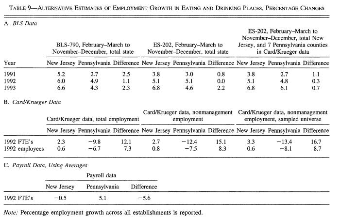
Card & Krueger (2000) published their reply in the same issue of the American Economic Review. They began by analyzing a new dataset, which consisted of BLS data for individual fast-food restaurants for the same counties as examined in their original study (and, by extension, in Neumark & Wascher’s), with the addition of seven more counties in Pennsylvania. Their results are best depicted in the following table:
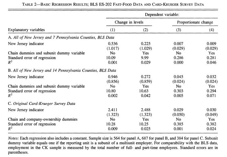
These effects are small and not even close to being statistically significant. The best estimate from this study (0.225 additional employees due to the increase) is a tenth of the best estimate from the original study (2.49 additional employees).
The next part of Card & Krueger’s response was a reanalysis of Neumark & Wascher’s data by constructing their own, more complete dataset. They found that Nuemark & Wascher’s sample was not random, and, specifically, biased toward inclusion of businesses with lower growth rates over this period. When Card & Krueger replicated their results, and added some controls, the results were no longer significant, and the effect size was miniscule. Furthermore, when they restricted the sample to the 48 fast-food restaurants in Neumark & Wascher’s sample which they could match with restaurants in their own sample, the results showed either no change or a slight increase in New Jersey employment relative to Pennsylvania.
Based on what they wrote in their book Minimum Wages (2008), Neumark & Wascher seem to accept Card & Krueger’s conclusion that the best evidence indicates that the rise in minimum wage in 1992 had a small and insignificant effect on New Jersey employment relative to Pennsylvania. So, to summarize, Card & Krueger originally concluded that there was a huge increase in employment due to the minimum wage; then, Neumark & Wascher conducted their own analysis, finding a small negative effect; finally, Card & Krueger conducted a superior analysis of a more complete version of the same data, and found that there was no significant effect, to which conclusion Neumark & Wascher seem to have agreed.
2.1a.2. California, 1988
In 1988, the Californian minimum wage rose from $3.35 to $4.25, which affected approximately half of all teenagers due to their wages being lower than the new minimum. Card (1992a) analyzed data for teenage employment in California alongside several bordering states between 1987 and 1989, who were not affected by any minimum wage increases during this time. Card estimated that the wages of teenagers living in California increased by about 10% during this period relative to the same demographic in the control group. The effect on employment was an increase of 5.6%, which was statistically significant (p<0.02). Once again, this early study actually found a positive effect of the minimum wage!
Kim & Taylor (1995) attempted to replicate these results by examining the retail industry specifically. The comparison group was the rest of the U.S. rather than just the states bordering California. While focusing on a specific low wage industry is probably better than examining all teenage employment,3 the control group is likely inferior to the one used by Card. Kim & Taylor estimated the impact of the minimum wage by finding the effect of the difference between the change in the average wage of an industry in California versus the rest of the U.S. The coefficient for this variable, which was equal to about -0.9 (two different models with roughly the same effect size, both p<5 × 10⁻⁸). This is in sharp contrast to Card’s estimated elasticity of over +0.5. It should be noted that Taylor & Kim also confirm their estimate by examining the effect of the Californian minimum wage increase by exploiting the fact that its effect would have been larger in magnitude for locations with initially lower average wages (this type of study will be examined in detail in 2.3). Their confirmation shows a similar elasticity of about -0.7 (p<0.001).
In their book, Card & Kruger (1995, pp. 101-108) criticize Kim & Taylor’s methodology, claiming that the disparity between Card’s and Kim & Taylor’s result is caused by measurement error in the data used by Kim & Taylor, which, given their specification, biases results toward -1 rather than 0. The reason for this is that average wage per worker was computed by dividing the total amount of wages paid in the first quarter of each year by the number of people earning a wage on the last day of March. This means that employment as of March 31st is mechanically negatively correlated with the average wage. In the original paper, Kim & Taylor found that there was often a highly negative correlation between their wage and employment change variables in most of the models for the year-long periods leading up to the minimum wage increase, though these were never significant, except for in one model for 1985-86, where the effect size was much smaller (-0.361). Card & Krueger analyzed the data for 1989 to 1990 using Kim & Taylor’s method, & found that these were negative, too, though, as Neumark & Wascher (2008, p. 303, n. 31) noted, these could have been caused by “a lagged effect from the 1988 increase”.
Most important was the reanalysis by Card & Krueger of the California increase’s effect, using the same DiD approach as employed by Card (1992a), but looking at workers in the restaurant and retail industries, rather than all teenagers in the state. The control group was, once again, restaurants in states bordering California, who did not experience a change in their minimum wage. For the retail industry, the DiD effect sizes, for comparisons of 1987 vs. 1989 and 1988 vs. 1989, were -1.26% and -0.29%, respectively. For restaurants, the same figures were +0.04% and -1.91%. Unfortunately, standard errors were not presented, so it is not possible to test for significance. A reduction of around 1% in employment would correspond to an elasticity of -0.12 for the restaurant industry (for the change in wage, see Table 3.6) and -0.20 in retail.
Lastly, I should note that Kim & Taylor’s analysis of the differential impact of the minimum wage across counties has also been criticized, and, in this case, whether or not there is a major problem is not ambiguous (see Kennan, 1995). However, this was never their primary measure, and also isn’t the subject of section 2.1.
2.1a.3. Texas, North Carolina, and Mississippi, 1991
Two studies examined the effect of the 1991 federal minimum wage spike to $4.25 an hour using the case study approach, and they reported their basic results in terms of elasticities. Katz & Krueger (1992) studied the impact on Texas by seeing if businesses more impacted by the minimum wage—because their starting wages were further below it—experienced different changes in employment afterward. They found that the fast food restaurants more impacted by the increase actually had an increase in both overall and FTE employment. The results, in terms of elasticity, were +1.73 (insignificant) and +2.48 (significant). As far as I am aware, these findings have not been challenged, unlike the other Krueger/Card studies.
Using basically the same method, Spriggs & Klein (1994), looked at two cities, one in Mississippi and the other in North Carolina. Their estimated elasticity was much lower (+0.062) and was nowhere near statistical significance.
2.1a.4. Pennsylvania, 1996-1997
In 1996, the federal minimum wage was increased to $4.75, and then in 1997 to $5.15. Recall that, in the most famous case study, the event was an increase in the New Jersey minimum wage to $5.05, relative to Pennsylvania, whose minimum did not change. When the federal increase occurred, the Pennsylvania minimum increased by $0.90, while New Jersey’s only increased by $0.10, the two states now being completely equal. This fact was used by Hoffman & Trace (2009) to explore the impact of the minimum wage on employment, this time using Pennsylvania as the treatment group, and New Jersey as the control. Their effect size estimate was an insignificant decline in teenage (16-19) employment of 3.76%.
2.1a.5. Illinois, 2004 & 2005
In January of 2004, Illinois raised its minimum wage from $5.15 to $5.50, and then to $6.50 a year later. This natural experiment was studied by Elizabeth Powers, Ron Baiman, and Joseph Persky in an unpublished report to the Russell Sage foundation. The authors of the report have published assessments of their findings, disagreeing in their interpretation of the facts. The design of the study was very similar to several of the other studies reviewed thus far: interviews were conducted at three separate times, before and after each increase, with Arby’s, Burger King, KFC, McDonald’s, Subway, Taco Bell, and Wendy’s restaurants in Illinois as well as in the control state, Indiana.
Powers (2009) was the first to describe the results of this study publicly. The main analysis was made up of a comparison between the first and third waves, as the second wave affected only about one third of the restaurants sampled (because most restaurants already had starting wages above the new minimum). Powers found a marginally statistically significant (p<0.1) reduction in FTE workers4 in Illinois compared to Indiana when comparing 2003 and 2005 interview data, and a statistically significant negative effect when comparing 2004 and 2005 in a supplemental analysis (Table 6). The losses were equivalent to about a reduction of 3 FTE workers, or, in relative terms, a drop by roughly 25% based on the 2003 baseline. Powers concluded that these data showed that the minimum wage has a strong negative effect on employment.
Persky & Baiman (2010) disagreed with Powers’ conclusion. They calculated a decline in Illinois relative to Indiana of either 0.88 or 3.1 FTE workers, depending on how an FTE worker was defined. The former figure represents the number of FTE employees as calculated in the same way as Card & Krueger (i.e a worker categorized as part time by the interviewee is counted as 0.5 FTE workers), while the latter is calculated in the same way that it was calculated by Powers, based directly on hours worked (see my fn. 6). The decline in the Card-Krueger definition of FTE employees was not significant even at the ten percent level, while the second definition was significant at the five percent level. The latter definition is preferable because it is a purer measure of hours, which is how labor is typically defined in employment schedules. So far, the results are concordant with those reported by Powers. However, Persky & Bainman also reported that adding a covariate for length of the pay period reduced the decrease in the second type of FTE worker to 1.9 workers, which made it no longer significant, though still large in magnitude.
2.1a.6. New York, 2004 & 2006
In 2004, the minimum wage in the state of New York was $5.15, which number increased to $6.75 in 2006. The first researchers to study this spike were Joseph Sabia et al. (2012). The comparison group consisted of three states: Pennsylvania, Ohio, and New Hampshire. The measure of employment was the employment rate of teenagers (aged 16-19) without high school degrees. The DiD estimated decline in the best model (Table 3, column 6) was 7.2 percentage points, or a relative decline of a little over twenty percent. This decline was just barely statistically significant (p= ~0.046).5 The later investigations of this minimum wage increase are discussed in section 2.1c.
2.1a.7. San Francisco, 2004
Near the end of 2003, a law passed in the city of San Francisco increased minimum wage to $8.50 an hour, which was a 26% increase to the previous minimum of $6.75. The law took effect in February, 2004, and its impacts have been analyzed by Dube et al. (2007), who used the East Bay area near the city as a control. The total sample consisted of around 200 restaurants from San Francisco and roughly 100 from the East Bay.6 Most of the effect sizes for both the total number of employees and the number of FTE workers were positive (implying that minimum wage had a positive effect on employment), but none were significant at even the 0.1 level, despite being somewhat large.
2.1a.8 Santa Fe, 2004 & 2007
In mid 2004, the minimum wage in Santa Fe (New Mexico) increased from $5.15 to $8.50, and, in the begininng of 2007, up to $9.50; thereafter, the minimum wage was set to be adjusted for shifts in the cost of living. Justin Hollis (2015) explored the effects of these increases on low wage workers, from 2004 to 2012, using the city of Albuquerque as a control, because the minimum wage in Albuquerque did not change nearly as much during this period (from $5.15 in 2004, to $6.75 in 2007, with small increases thereafter). Low wage workers were defined as those in occupations where employees at the 75th percentile earned less than the 2004 minimum wage in 2003. In terms of total employment in these industries, there was an insignificant decline of 12.54% in the first increase (i.e., in 2004), and of 24.50% in the second (i.e., 2007). However, the first decrease is difficult to interpret, as the change in income was only marginally significant (p<0.1).
2.1a.9. Six Cities, 2009-2015
Allegretto et al. (2018) examined the effects of the changes in minimum wage in the following cities: Chicago, D.C, Oakland (California), San Francisco, San José, and Seattle—each of which had multiple increases over the period under study (2009-2015). A comparison group was used for each city; four comparison groups had no increase during the period of this study, while the other two had no real increase, but still had a nominal one, as their minimum wage was set to mimic shifts in inflation.7 Employment was measured in terms of total number of people employed. The authors summarize their findings in the following table, pertaining specifically to the food service industry (MW=minimum wage):8
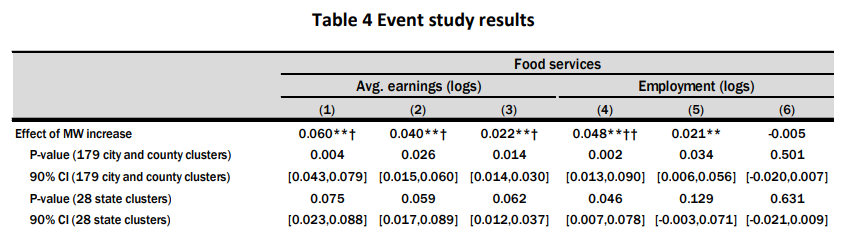
The relevant columns are three and six, as these control for population size, private sector size, and the economic trend before the change in minimum wage. These show a decline of about half a percent in employment, though this is not statistically significant (note: to read this table, just multiply the log values by 100, which gives you an approximately equal value in percentage terms).9
2.1a.10. L.A, 2016-2019
A wage ordinance passed in L.A in 2015 raised the minimum wage several times between 2016 and 2018, and the effects of these increases were studied by Wachter et al. (2020), who used similar locations near L.A as controls. This is their main table:
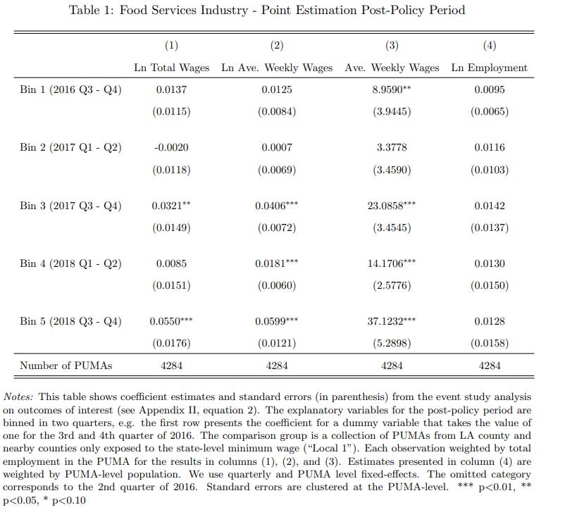
Each “bin” in the above table represents an increase in the minimum wage. Only two increases resulted in a statistically significant increase in overall wages, and only three in log average weekly wages. Because overall wage is never defined, while weekly wage is (p. 27, fn. 27), and because this is the measure focused on by the authors, I will use this one. In the three rows where the increase in weekly wages was significant, the effect on employment was positive, but never significant.
2.1a.11. California, 2024
Beginning April 1, 2024, California adopted a 20$ per hour minimum wage. The first preliminary report was published in October of the same year (Schneider et al., 2024). It found that there was a tiny increase in average weekly hours in the fast food industry relative to a control group of fast food restaurants in stated whose minimum wage did not change. A second report was published in July of 2025 (Clemens et al., 2025). These researchers found a decrease in employment, seemingly measured as the portion of people employed, of 3.5%.
The most recent report was published in September by Sosinky & Reich (2025). They examined the fast food industry specifically, and the control group was fast food restaurants in states near California who did not have their own increase. They found an employment effect ranging from around -0.8% to +1.2%, representing the portion of the population which is employed at fast food, depending on which quarter one uses. Because this final report uses a weird definition of employment and covers the same time span as the July report, I think that the estimate from the latter should be preferred.
2.1a.12. 288 Minimum Wage Spikes Between 1990 and 2006
Some studies have combined the effects of many events. The first of these was Dube et al.’s (2010) examination of 288 minimum wage changes between 1990 and 2006 among counties that border each other. Put simply, if a state increased its minimum wage, while a state bordering it did not, counties touching each other across that border would be compared. Their effect size in the best model was an elasticity of +0.085 for the restaurant industry, which does not attain anything near significance.10
These results were questioned by Jha et al. (2024), who argued that the county-pair approach used by Dube et al. was sub optimal. Instead, they compared counties within the same commuting zones, that is, counties between which there are a lot of work commutes. Among their arguments in favor of this method, these researchers noted that two of the three authors of the original paper (i.e., Dube et al., 2010) had previously written that the commuting zone approach is superior. Their semi-replication is summarized in the following table (DLR = Dube et al.):
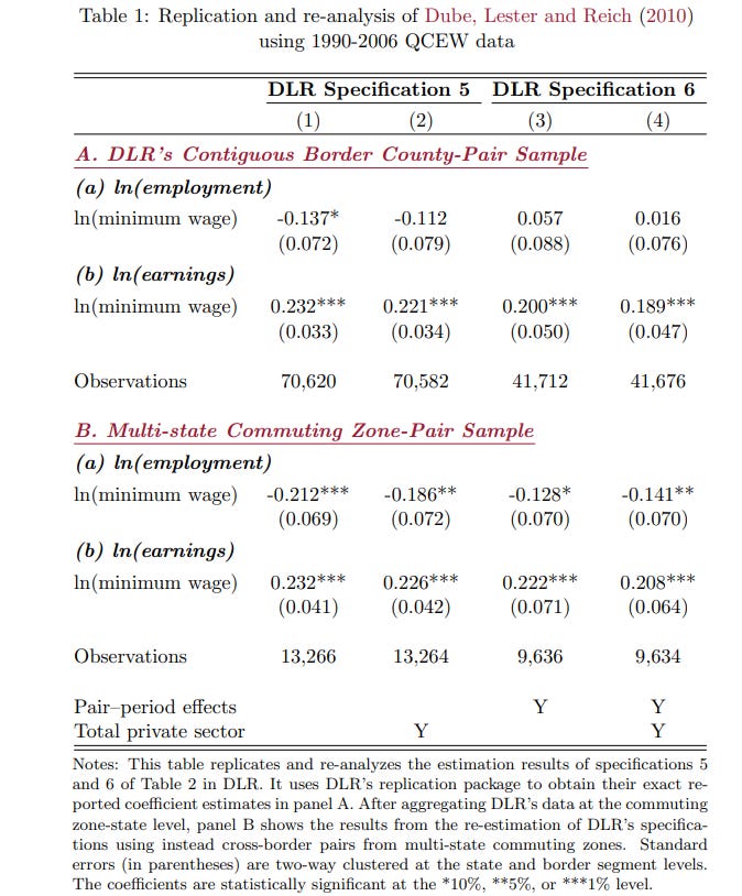
It can be seen that the employment effect reversed sign, became much larger, and obtained statistical significance. The elasticity was -0.68 with a p value of approximately 0.043. After this, Jha et al. went on to conduct their own analysis, which will be analyzed a little further down.
2.1a.13. 441 Minimum Wage Spikes Between 1985 and 2012
The next such study was Joan Monras’ (2019) study of all changes in state-level minimum wages between 1985 and 2012. Rather than using bordering county pairs as experimental and control groups, he used the low skilled and high skilled population of the same state. Because low skilled people are much more likely to be affected by the minimum wage, this should work, but it is probably inferior to the approach used by Dube et al. They report their results in terms of FTE workers, defining part time workers as half a full time worker.
The main table reported a decrease of 1.88% in the FTE employment rate of low skilled individuals (Table 3). This was statistically significant at a p value of about 0.035, which makes Monras’ study one of the only ones with statistically significant effects. Despite probably having a worse methodology than the similar one conducted by Dube et al., it is a much better in terms of statistical power.
2.1a.14. 138 Minimum Wage Spikes Between 1979 and 2016
Another such study was published in the same year by Cengiz et al. (2019), looking at 138 state-level changes in the minimum wage. The control group was jobs with wages that were slightly above the new minimum before it was implemented, while the experimental group was jobs with wages below the new minimum. Their DiD effect size was estimated by subtracting the change in the number of jobs which pay slightly below the new minimum from the change in the number of jobs which pay slightly above it. Put more simply, they did the following: 1) found the number of jobs paying below the new minimum that were lost after the new minimum was implemented; 2) figured out how many more jobs paying slightly above the new minimum there were after it was implemented than before; and 3) subtracted the first number from the second. If, after the increase, there were more sub-minimum jobs lost than sur-minimum jobs gained, the effect on employment is estimated to be negative. In their preferred model (Table 1, column 7), the effect on employment was positive, but insignificant, with an implied elasticity of +0.41.
2.1a.15. 7 Minimum Wage Spikes Between 2010 and 2018
This study, conducted by Dube (2019, technical appendix A), is almost exactly the same as the one that has just now been described, except with further controls. Between 2010 and 2018, seven states increased their minimum wage to some value above $10.50, while 21 states (plus New Mexico, which was excluded due to major increases in local minimum wages) maintained their minima at exactly the federal level during this period. His main table (A1) lists the elasticity estimates from various models—all are positive, but none are even close to significance. Because I genuinely cannot tell which specification is the best, I chose the second column due to its estimated elasticity being around the average of the other equally good models. The result in this column was an elasticity of +0.32, similar to the results from Cengiz et al.
2.1a.16. Minimum Wage Spikes Between 1990 and 2016
As mentioned in section 2.1a.12, Jha et al. (2024) also analyzed an original dataset. Their study consisted of changes in minimum wages both at the county and state level within commuting zones between 1990 and 2016. Their main results (Table 3, column 1) indicated a statistically significant decline in employment, and an elasticity of -1.29 (p= ~0.005).
2.1a17. Summary
Despite these studies often being cited as definitive proof that raising the minimum wage has no impact on employment, there are several problems with using these studies to support that conclusion. The most obvious issue is that all of these studies were underpowered, and so cannot reliably estimate a moderately negative effect even if it assumed that the true effect is negative. In Card & Krueger’s (2000) final analysis of the 1992 New Jersey minimum wage found a DiD effect size of 0.272 for the increase when the control group was businesses from fourteen Pennsylvania counties, with a standard error of 1.029. Using the standard formula, this indicates that the 95% CI was -1.745 to 2.289. Below is a table depicting the elasticity estimates, their standard errors, and their 95% CIs. The overall elasticity estimate is presented in the bottom row, excluding several of the estimates that pertain to multiple events to avoid overlapping samples.11 The pooled elasticity is -0.27, with a p value below 0.005.12
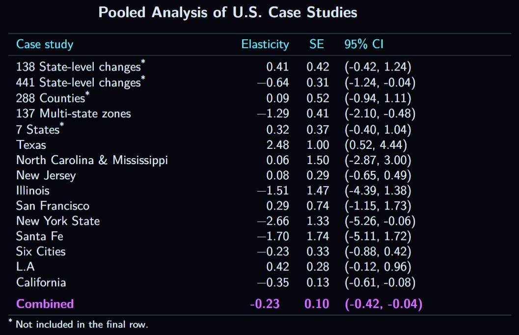
Overall, then, the U.S. studies which used this method, while inconsistent, come up with a highly significant negative elasticity when pooled. The point-estimate, -0.27, is not outside the traditional estimate of -0.1 to -0.3, and includes that entire range in its confidence interval.
2.1b. The Case Study Method: Studies Outside the U.S.
Studies from outside of the U.S. used much weaker designs because changes occurred at the national level rather than the state or local level as in the American studies. Therefore, the treatment and control groups are usually not as well defined.
2.1b.1. Cost Rica, 1988-2000
Gindling & Terrell (2007) explored the effect of changes in the minimum wage in Costa Rica between 1988 and 2000, by comparing workers in the covered and uncovered sectors. their estimates indicated that a 10% change in the minimum wage would decrease employment by 1.09%, which effect was marginally significant (p<0.1). Average hours of those remaining in the workforce in the covered sector also dropped, and the estimated loss was statistically significant, but the coefficient was actually about the same in the uncovered sector (not significant), making the evidence in this regard difficult to interpret.
2.1b.2. The 1990-1994 West Java Wage Spikes
In 1990, the difference in minimum wages between two bordering regions in Indonesia, Jakarta and West Java, was approximately 36%. However, between 1990 and 1994, the West Javan minimum wage increased so much that it bridged the gap entirely. Alatas & Cameron (2003) used detailed data of comparable businesses in both regions between 1990 and 1996 to examine the effect that the minimum wage increases between 1990 and 1994 had on businesses in Botabek (located in West Java) relative to Jakarta. The best estimates revealed mostly negative effects, depending on the size of the business and what the comparison years are. Because the biggest increase in the minimum wage in Botabek relative to Jakarta occurred in 1991 (see Table A1), 1990 should probably be used as the baseline year. If that is done, the effects are negative for small domestic and large foreign businesses, but positive for large domestic businesses. Weighing the results by sample size and combining them, there is a statistically insignificant reduction of 23.34 workers per firm, equivalent to a decrease of 5.5%.13
2.1b.3. Western Australia, 1994-2001
Between 1994 and 2001, there were several minimum wage spikes in West Australia. In order to estimate the effects of these spikes, Andrew Leigh (2003) compared employment changes among West Australian workers after each spike to workers residing in the rest of Australia. When the effects of all of these increases were put together, the elasticity of employment relative to the minimum wage was estimated to be -0.13, meaning that a ten percent increase in the minimum wage would decrease employment by a 1.3%. This effect is highly statistically significant (p= ~0.0021). However, when disaggregated by age groups, only the coefficient for 15 to 24 year-olds remains significant at conventional levels (elasticity of -0.389; p<0.005). Because youths are typically the group examined for this type of analysis, though, this result is not very surprising.
2.1b.4. New Zealand, 2001
In 2001, New Zealand increased its minimum wage for teenage workers. Hyslop & Stillman (2007) explored the effects of this change by using a comparison group of workers aged slightly above the cutoff (i.e., 20 and older). In their most basic DiD estimates, where the effect size is equal to the employment change for 16-17 and 18-19 year-olds minus the change for 20-25 year-olds, the estimated change in employment is positive for both teenaged groups, though not close to significance for either. A more intricate analysis with controls was also provided. In the best model (Table 4, column 7), the DiD estimates were negative for both groups of teenagers, though none are statistically significant.
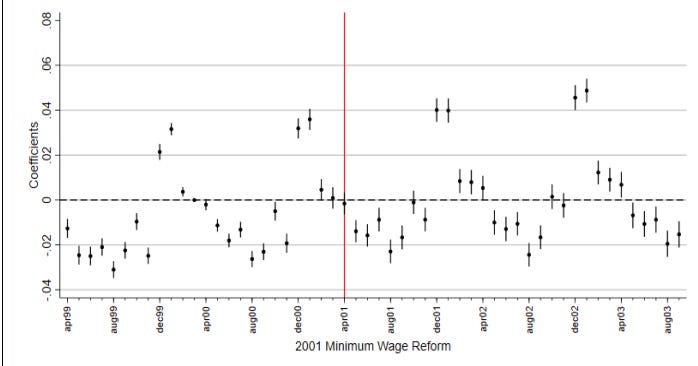
This analysis was replicated by van der Westhuize (2022) using the same methods but with better data. Using the simple DiD approach, he found, similarly to Hyslop & Stillman, a positive effect on both groups of teenagers, though, unlike the prior study, the effect was highly statistically significant. In the regression results, all of the estimates were still positive, but smaller in magnitude (Table 5, column 13); all were highly statistically significant. However, the author noted that tests of parallel trends—that is, tests to see if 20-25 year-olds and teenagers had similar employment patterns before—showed that, even before the change in the minimum wage, shifts in teenaged employment did not track shifts in young adult employment. This was shown in two figures, each including all of the controls used in the main regression model (i.e., Table 5, column 13). To avoid redundancy, I only show the trend analysis for the 16-17 year-old age group below. Clearly, the parallel trend assumption was violated, making DiD analyses untenable.14 The author concluded that, despite the strong looking regression results, “the true effects on employment remain uncertain” p. 26).
2.1b.5. New Zealand, 2008
Seven years later, New Zealand enacted another teenager-specific minimum wage increase, though, this time, only for 16-17 year-olds. Using the exact same method as before, Hyslop & Stillman (2021) found statistically insignificant negative results when using a basic DiD model, and tiny, insignificant coefficients with varying signs in the more complex regression model (Table 4, column 9). However, parallel trends were not tested for here, which may mean that the problem identified with the earlier analysis may apply here, too. A much bigger issue, however, is the fact that the estimated effect on weekly income is insignificant and/or negative in most of the year-specific coefficients (Table 7)! Clearly, not much, if any, weight should be placed on this study.
2.1b.6. The 2003-2012 Brazil Minimum Wage Spikes
Saltiel & Urzúa (2022) analyzed all changes in the minimum wage in five Brazilian states between 2003 and 2012, with the control group being a bordering state. Specifically, they examined the restaurant and accommodation industries. Their best model showed a slightly positive, but nowhere near significant, impact on employment (Table W2, column 8).
2.1b.7. The U.K., 2011-2019
In the United Kingdom, local councils are allowed to set living wages, which are above the minimum wage. Datta & Machin (2024) compared areas that had a higher minimum wage (i.e., a living wage ordinance) to those that only had the national minimum wage, using data from a large company with locations throughout the U.K. They found a positive, but only marginally significant, effect on entry level employment.
2.1b.8. Summary
Below is a table summarizing the non-U.S. data, though, unfortunately, with only three estimates:15

While the point-estimate is positive, the confidence interval is so wide as to once again include the entire traditional range of -0.1 to -0.3. On its own, the non-U.S. data does not provide much evidence against the old consensus.
2.1c. The Case Study Method: Synthetic Control Studies
All of the studies reviewed in sections 2.1a and 2.1b used natural controls—either workers/businesses/jobs not affected by the minimum wage change, or nearby states that were not affected. Another approach is to use a synthetic control, in which data from many possible controls are put together, to create a hypothetical control that is very close to the treatment group before the minimum wage increase. In practice, this is usually done by taking a change in one state, and then combining data from all states which didn’t have a rise in their minimum wage, weighted such that the hypothetical control state you created most closely matches the treated state in terms of whichever variables you choose to include; states which are used to make the synthetic control are called donor units. The biggest issue with this method is that there is no way to account for unobservable characteristics, which is one of the main reasons that natural controls were promoted by the New Economics in the first place.
However, as critics of the New Economics have pointed out, there was never much reason in the first place to believe that bordering states are the best control group. For example, Neumark et al. (2014) wrote, “nothing in the Card and Krueger study establishes that Pennsylvania is a good—let alone the best—control for New Jersey” (p. 621). Indeed, in many comparisons, there was a sizeable difference between the treatment and control group in terms of its observed characteristics before the spike, and observable differences should surely be expected to matter more than unobservable ones when state-level economic statistics are so thorough. This was demonstrated in the same paper by Neumark et al. (Table 3), which found that the synthetic approach placed the vast majority of its weight on donor units outside of the same Census Division (i.e., only between a quarter and a third of the total weight was, on average, placed on states within the same region for a given variable, which is only about two to three times as large as chance, given that there are nine such divisions). The synthetic approach appears to be supported by researchers in the New Economics, and has been employed in several studies that used the case study approach.
2.1c.1 The 2005-2006 D.C Minimum Wage Spikes
As reviewed in section 2.1a.5, Sabia et al. (2012) explored the employment effect of the large New York minimum wage increase between 2004 and 2006, and found a statistically significant decline in employment. In the same paper, they also used a synthetic control with seven states acting as donor units. They found a larger employment decline with this approach than when they used a natural control, though the standard error was much higher, and the result was only marginally significant (p<0.1). However, calculating the elasticity was not possible, because change in the average wage was not calculated.
Fortunately, this study was soon criticized by Hoffman (2016), who tried to replicate it with a more complete version of the same dataset. He found a smaller effect on employment, and this effect was no longer significant. This led Sabia et al. (2016) to redo their synthetic analysis using the same dataset as Hoffman. They found that the states they used as controls were, based on their weights in the synthetic control, not very good. More importantly, their synthetic DiD estimate found approximately the same effect size on employment, at almost the same p value (~0.07 vs. ~0.046) as in the natural controls in the original analysis, though it is not possible to calculate the elasticity because they did not compute the effect on average wages.
In the same article, they also provide estimates for several other states as well as D.C,16 and, in those cases, do provide wage-change data. All of these had a large increase in their minimum wage between 2004 and 2006. Unfortunately, however, the increase in wages for 16-19 year-olds without a high school degree was only statistically significant in the case of D.C (all of the other states’ effect sizes were tiny, not just insignificant), so that is the only location that is possible to analyze. These changes, according to Google, occurred in 2005 and 2006, with increases to $6.60 and $7.00, respectively, from $6.15 at the start of the period. There was an estimated rise in employment of about 4.62%,17 which does not attain anything close to significance.
2.1c.2 Minimum Wage Spikes in Six Cities Between 2009 and 2015
Nadler et al. (2019) provide synthetic estimates for each city in the study previously analyzed in section 2.1a (Algretto et al., 2018). Unlike that study, which only reported the aggregated outcome, Nadler and his team report outcomes for each city separately. Of the six cities, four had a statistically significant increases in income; these were Oakland, San Francisco, San José, and Seattle. One city (Oakland) had a statistically significant positive effect on employment, while the other three had very small and insignificant effects.
The Seattle data has been analyzed in a more detailed way by Jardim et al. (2022). For their donor units, Jardim and his team used localities in Washington but outside King county (where Seattle is). Because there were two increases, one to $11 in 2015, and the other to $13 in 2016, their results can be used to calculate two different elasticities. The former elasticity estimate is -0.77, but nowhere near significant(p= ~ 0.43). The latter, on the other hand, is even more negative, at -1.95, and is now significant (p<0.01).18 Both elasticities are based on hours.
2.1c.3 The New York and California Minimum Wage Spikes Between 2013 and 2019
Wiltshire et al. (2024) used state level changes in the minimum wages of New York and California between 2013 and 2019, specifically looking at the 36 counties with the highest population. The synthetic control was based on 122 counties that stayed at the federal minimum wage during the entire period. Their main table’s best model shows a statistically insignificant decline in employment of 0.22%.
2.1c.4 28 State-level Minimum Wage Spikes Between 1979 and 2013
Dube & Zipperer (2015) used the synthetic control approach to measure the effect of 28 difference minimum wage increases between 1979 and 2013. None of the states’ employment changes were statistically significant using even an alpha of 0.1 (Table 5), and neither was the combined effect. The pooled elasticity was -0.16, with a 95% CI of (-0.54, 0.21).19
2.1c.5 The 2015 Germany Minimum Wage Spike
In the beginning of 2015, Germany raised its national minimum wage to €8.50 per hour. The effects of this minimum wage were assessed by Hakobyan (n.d), who created a synthetic control using data from eight OECD nations which had no minimum wage and were sufficiently developed. Because some industries were given about two years of leeway before the minimum wage became binding, employment effects were assessed as of the second quarter of 2017. Employment was measured as the employment rate of those aged 15 to 24. The finding was that the minimum wage reduced employment by 4.79 percent. Unfortunately, this study could not be included in the summary results because data regarding SE and change in average wages were not reported.
2.1c.6 The 2019 Spain Minimum Wage Spike
Roughly the same method was used by Arnadillo et al. (2024) to study the effects of the national minimum wage increase in Spain, which occurred in 2019. They found essentially no effect, but, again, these results could not be included in the summary statistics because they did not report change in wages or the standard error.
2.1c.7. Summary
Unfortunately, I could only find four studies whose data could be included in the summary table, all of which come from the U.S., with a total of eight different estimates. Below is a table summarizing the results:20

Unfortunately, it was not possible to pool these studies, due to their standard errors not being comparable, as synthetic studies require permutation-inferred SEs and different studies handled this in different ways. The overall unweighted average was -0.16, while the median was -0.02, with the latter probably being a better summary statistic.
2.1d. The Case Study Method: Overall Summary
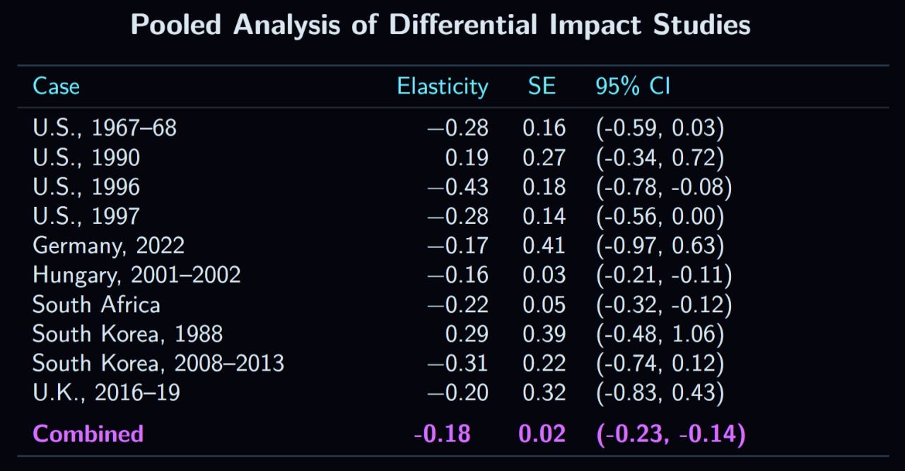
In all, case studies were remarkably inconsistent, because of their low precision. Combining all three sections—the U.S., non-U.S., and synthetic data—there were 32 estimates, of which 18 were positive, 13 were negative, and one was inconclusive. Of those studies finding significant results, however, the ratio is much less even: six negative and two positive. In order to get a better idea of the true effect, I combined all of the elasticity estimates, for a total of 15 elasticities with standard errors. A table summarizing each elasticity estimate would be too large to include here, the data is represented in the following chart instead:
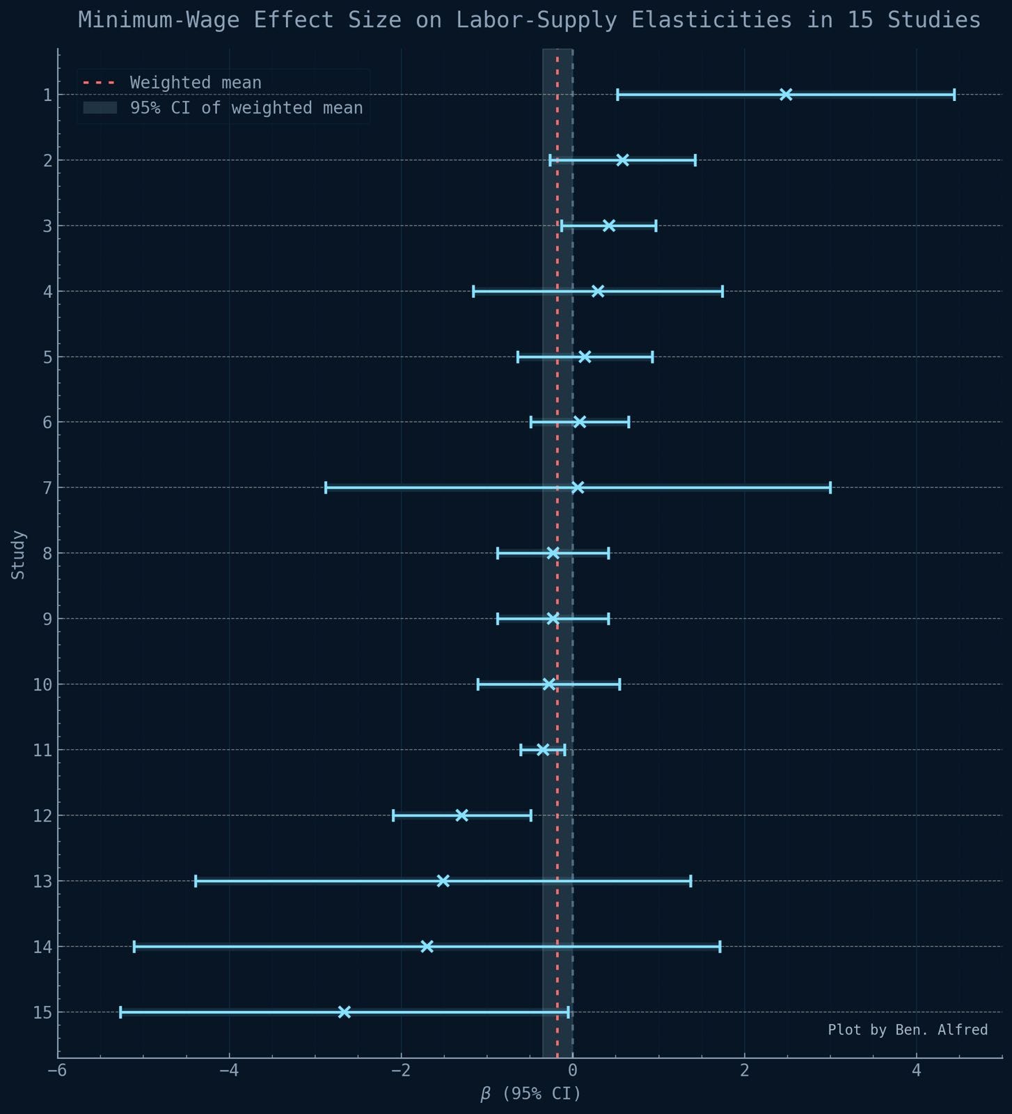
The average elasticity, weighted for SE, which is colored red, was -0.18, with a 95% CI ranging from -0.36 to 0. The effect is just barely insignificant (p= ~0.0504). Unfortunately, the literature is simply too imprecise to give a useful point-estimate. When I estimated the power of each of the studies (including overlapping samples, but not including the synthetic control studies) to detect an elasticity of -0.2 (i.e., the probability that they would find a significant negative effect if the true effect were -0.20, based on their SEs), none met the typical threshold of 80%! The average power was just 13%, while the median was 12%. Clearly, the state of this literature is very poor, and it is not surprising that so many researchers in the New Economics have concluded that the effect is either positive or null.
2.2. The Differential Impact Method
In this method, the effect of a given minimum wage increase is estimated by comparing regions, or, in some cases, industries, which are differentially affected by the increase. The differential impact is estimated by the portion of workers with wages below the new minimum wage, or, in some cases, the ratio of the new minimum to the average wage in a location. The impact of the minimum wage is typically referred to as its “bite”, whichever way it is measured. For simplicity, I will only review national increases here, excluding a few county-level analyses of state-level increases in the U.S.
2.2.1. U.S., 1990
The first study to implement this methodology was published by David Card (1992b),21 and was based on the the 1990 federal increase from $3.35 to $3.80. According to him, the portion of teenager workers earning less than the new minimum before it went into effect ranged from “under 10% in New England and California to over 50% in many southern states” (p. 22). Therefore, there was considerable variation in bite. Card categorized states as either low-wage (and therefore high bite), medium-wage, or high-wage, and found that all categories of states experienced increases in hourly wages and drops in their teenage (16-19) employment rate between 1989 and the same quarter of 1990. Because the increase occurred in April, there were three post-treatment quarters. Card concluded that his analysis showed that the federal increase had no effect or, if anything, increased employment, as the overall employment loss was lower among low-wage states than high-wage states. However, using the same data, one could reach a different conclusion. By adjusting for the change between the first quarter of 1989 and 1990, during which data would reflect a pre-minimum wage growth trend, I got the following changes: -14.38% for low-wage states, -8.16% for medium-wage states, and -0.60% for the high-wage states.22 This is because the pre-treatment trend was already such that lower wage states were gaining employment much more quickly than the medium-wage states, while the high-wage states were losing it. These numbers should be interpreted with caution because the low-wage employment change (not the adjusted change, but the one presented by Card) was not statistically significant, and the other two categories’ changes have very wide confidence intervals.
Next, Card moved onto a much better analysis, where he examined state-level changes (including D.C) as a function of the fraction of teenagers affected by the minimum wage (the same criterion as he used to sort the states into wage categories). In the best specification, he found an insignificant elasticity of +0.19, though this again did not adjust for pre trends; though perhaps much of the pre-trend effect, if there was one, would have been accounted for by controlling for changes in overall employment, which Card did do, making such an adjustment unecessary.23
2.2.2. The 1967-68 U.S. Minimum Wage Spikes
In 1966, legislation was passed that increased the U.S. minimum wage by 28% in two phases—first in February, 1967 and again in February, 1968), and expanded its reachto millions of more workers, as part of Lyndon B. Johnson’s War on Poverty. Bailey et al. (2021) evaluated the effect that this change had on men aged 16 to 64.24 The bite was determined by the share of a state’s workers earning less than the second increase (i.e., the one in 1968) in 1966. In the U.S. as a whole, a little over 16% of workers were earning less than the new minimum, with state-level variation from slightly less than ten to a little over thirty percent. In the best model (Table 3, column 4), the elasticity was -0.28, but only marginally significant, for hours worked.
2.2.3. The 1996 and 1997 U.S. Minimum Wage Spikes
In 1996, the U.S. federal minimum wage was increased from $4.25 to $4.75, and, in 1997, to $5.15. Both changes were studied by Thompson (2009) who, rather than using states as his unit of analysis, used county-level data. High and low impact counties were defined by the mean teenage earnings. Three different estimation strategies were used: 1) comparing counties in the top fifth of the teen wage distribution to those in the bottom fifth; 2) contrasting those in the top third to the bottom third; and 3) using a continuous treatment. Probably, the last of these is the best measure of bite. The continuous measure serves as a form of inverse bite, as it regresses an additional $100 in mean teen quarterly wage on the impact of the spike. While the coefficient for this variable on employment was very small, it represented an elasticity of about -0.43 for the 1996 spike and -0.28 for the latter increase.25
2.2.4. The 2003-2012 Brazil Minimum Wage Spikes
Between 2003 and 2012, the Brazilian minimum wage grew by almost two thirds in real terms, according to Saltiel & Urzúa (2022), whose paper I already analyzed above in section 2.1b.6. Here, I focus on a different analysis by the same authors, which exploited the regional variation in bite from these increases, measured by the ratio between the median wage of a state and the new minimum wage. These researchers found a statistically insignificant decline in employment, which, unfortunately, cannot be converted to an elasticity because of a lack of wage data.
2.2.5. The 1981 France Minimum Wage Spike
In June of 1981, the French minimum wage increased by ten percent. In order to assess the impact of this change, Bazen & Skourias (1997) examined the shift in teenage employment between march and October of that same year, looking at 32 sectors, and measuring bite in terms of the portion of workers affected by the increase. In order to account for seasonal differences, a DiD approach was used, wherein the coefficient on the bite variable was adjusted by coefficient it would have had in 1980 (a form of pseudo event test). The effect was negative and large in magnitude, but nowhere near achieving statistical significance. The authors also examined the effects of further increases in the French minimum wage after 1981, but used the same bites for each sector, estimated based on the 1981 minimum wage, and so their results are difficult to interpret; I do not include the findings of this latter analysis in my summary.
2.2.6. The 2015 Germany Minimum Wage Spike
Bruttel (2019) has written a literature review summarizing evidence coming from Germany’s first ever implementation of a national wage. In terms of employment effects, he cited five studies that found a negative employment effect, one that found a positive effect, and another that found a negative effect only for youth employment, but a positive effect for the economy overall. All but one of these used a disparate impact approach, and, here, I will review those.
Ahlfeldt et al. (2018) found, using 401 county-units, and exploiting variation in bite, that a 1% increase in the minimum wage was associated with an increase of wages at the tenth percentile by half a percent, and employment by 0.06%, with an elasticity of 0.12. The increase in employment was statistically significant (p<0.05). On the other hand, Caliendo et al. (2018) estimated a large decline that was significant, using two different measures of bite, one based on the fraction of workers earning less than the new minimum, and the other based on the ratio of the minimum wage to the average wage (p<0.05 and <0.01). The main difference between this study and the last one is their inclusion of much better controls. An elasticity could not be estimated because of the lack of wage data.
Alfred Garloff (2017) used data from 141 labor regions, and found a significant decline in employment (Table 2, Panel B; p<0.05).26 However, many of the more specific models have insignificant or positive effects. Once again, there was no income estimate, so the elasticity could not be estimated. Holtemöller & Pohle (2017) used a few hundred state-industry units, but did not present their results in an easily interpretable manner, though they conclude that the effect was negative on “marginal” work (i.e., part time, low-wage labor) but positive on other forms of employment. There were no wage data.
Schmitz’s (2017) study provides more detail. Using data for 402 counties, he found a consistently negative effect of bite on employment which was statistically significant in three out of four of the regressions for “regular employment” and for all four for marginal employment. Bruttel (2019) reasonably summarized this paper as showing a decline of around 0.1% in regular employment and 1 to 1.4 percent in marginal employment. Once again, it was not possible to calculate elasticity. There were no other English-language publications included in Bruttel’s literature review.
Because the only study where it was possible to calculate the elasticity did not provide the standard error, there is no usable data for this minimum wage spike. However, it can be safely said that the best available evidence suggests a statistically significant negative effect (Caliendo et al., 2018).
2.2.7. The 2022 German Minimum Wage Spike
Several years later, Germany increased its minimum wage again. In a study published by Bossler et al. (2024), bite was defined as the fraction of workers in a given county that were below the new minimum wage before it was put into effect, and the unit of analysis was 400 counties. The effect on the overall employment rate was negative but small and insignificant (Table 2, column 2, November and December). Unfortunately, the income change using this exact method was not reported, but using an alternative method, described in a different part of the same paper, the change was calculated as about +5.7%. This gives an elasticity of -0.17, but, once again, it is not significant.
2.2.8. The 2001-2002 Hungary Minimum Wage Spikes
In 2001, Hungary raised its minimum wage by about 57%, and, in 2002, by another 25%. Harasztosi & Lindner (2022) examined the change in employment caused by these two spikes by comparing firms with different proportions of their employees earning beneath the 2002 minimum wage. The short term effects are measured using the coefficient for fraction affected for the changes from 2000 to 2002, while the medium term effects are estimated for the years 2000 to 2004. They find that the estimated decline for a firm whose employees were all earning below the 2002 minimum wage relative to ones whose employees were all earning above it was 7.6% in the short term, and 10% in the long term. Both of these were highly statistically significant (both p<5 × 10-14).
2.2.9. The 2004-2018 Poland Minimum Wage Spikes
In Poland, there is no local variation in the minimum wage, and the national minimum wage is set each year. These changes have been analyzed using bite variation between localities by two different teams of researchers—Majchrowska & Strawinski (2021) for 2006 through 2018, and Albinowski & Lewandowski (2022) for 2004 through 2018.
The first team of researchers defined bite as the ratio of the mean wage of a labor market (of which there were 380) and the national minimum wage. They found a negative relationship between employment growth and bite, indicating that the minimum wage reduced employment, though the effect was not close to significance in any model. The authors found that the estimated bite coefficients varied by year, but none of the by-year differences were statistically significant. Elasticity could not be calculated because of the lack of information regarding wages. The second team used 73 subregions, and calculated bite in the same way as the previous analysis. They found that bite actually had no relationship with wage growth rate in the full sample of regions, indicating that the minimum wage did not raise wages at all—which obviously cannot be true. When analyzing the effect in regions with mean wages in the bottom third of the sample, there was a statistically significant increase in wages and decline in employment, which implied an elasticity around -0.38 (p. 12). However, I do not feel comfortable relying on this study due to the weird full-sample results.
2.2.10. The 2003 South Africa Minimum Wage Spike
In March of 2003, the South African minimum wage increased, but only for certain industries. One of these industries was farm labor. Bhorat et al. (2014) exploited the fact that some industries were not affected by this change to estimate its effect. Their treatment group was unskilled farm labor, which was covered by the increase, and their control group was described as “unskilled, nonunionised individuals of working age, who are not covered by another sectoral minimum wage” (p. 3). They then calculated the DiD effect size for wages and employment by comparing these two groups before and after the change, controlling for district, and using the minimum wage to average wage ratio as the bite measure. Their results suggested that farm worker wages rose relative to the other unskilled workers’ wages by 25.11% (Table 5).27 The change in employment, measured in terms of the proportion of workers in the sample who are employed as farm laborers, is -5.47% (Table 4).
2.2.11. The 1988 South Korean Minimum Wage Spike
The first national South Korean minimum wage went into effect in the beginning of 1988, applying to all factories employing ten or more workers. Baek & Park (2016) studied the effect that this increase had on employment at these factories, using plant-level bite, defined as the difference between the pre-implementation mean wage at that factory and the new minimum. The effect size was positive but nowhere near significance.
2.2.12. Spain, 1967-1994
Dolado et al. (1996) examined changes in the Spanish minimum wage between 1967 and 1994, using the ratio between the average wage and the minimum wage for each region as the independent variable. These authors found a statistically significant positive relationship between the bite index and employment change over the whole age distribution (p<0.00002). When limited to just teenagers (16-19), the coefficient became negative, though only marginally significant, despite having twice the magnitude of the significant effect on overall employment (p<0.1). Furthermore, the same researchers examined in detail a 1990 change in the law, which made it so that the 17 year-old minimum wage also applied to children aged sixteen and younger, and also slightly raised the minimum for 17 year-olds. This resulted in a large increase in their minimum. Based on interregional variation, the bite index (now the fraction paid below the new minimum) had a negative coefficient for those aged 16-19 (unfortunately, sixteen year-olds could not be separated from those aged 17 and older), but was positive for those slightly older (20-24). The point-estimates for both seem somewhat high in magnitude, though standard errors were not given. In my opinion, the best conclusion from this paper is that the minimum wage reduces teenagers’ employment, but probably has a positive effect on older age groups’ employment.
2.2.13. The 2008-2013 South Korea Minimum Wage Spikes
South Korea increased its minimum wage each year from 2008 to 2013. Lee & Park (2025) analyzed the effects of these increases by using firm level data and a bite variable equivalent to the fraction earning at or above the old minima but below the new minima in each successive year. The effect on employment was negative but insignificant.
2.2.14. The 2016 U.K. Minimum Wage Spike
In 2016, the United Kingdom spiked its minimum wage to £7.20, and afterward increased it regularly. The effect of these increases through 2019 were studied by Giupponi et al. (2024), who measured bite in terms of regional differences in average earnings. Change in employment was estimated in the same way as in a study reviewed previously in section 2.1a.14 (Cengiz et al., 2019), and, because only those aged 25 and older were affected by the increase, only their employment was measured. Giupponi et al.’ main specification found an insignificant elasticity of -0.20, with essentially the same results for alternative regressions.
2.2.15. Summary
With a total of 10 elasticity estimates, the conclusion is largely the same as for the case studies:28
The pooled effect size is -0.18, with a p value below 1 × 10-13. Clearly, this method also gives results consistent with the traditional estimate.
2.3. The Longitudinal Method
The final method that I analyze in section 2 is the longitudinal method. In these studies, two groups of individuals are assessed in multiple waves—one control group and one treatment group—and their employment trajectories are compared. The initial wave occurs before the minimum wage increase, and the follow up occurs after an increase. The longitudinal method is intuitive because it directly compares individuals instead of cross sections of individuals or municipalities, and has been used in many studies of the minimum wage’s effect on employment, though not in as many as the case study approach.
2.3.1. U.S., 1975 & 1980-1981
This section reviews the two studies cited in Card & Krueger’s overview of this method (1995, pp. 223-231). The first was an analysis of the 1975 minimum wage increase to $2.10 from $1.60, conducted by Ashenfelter & Card (1981), and published as a discussion paper in 1981, but I cannot find this paper anywhere (hence why it is not linked in the in-text citation, though it is included in the reference list). On David Card’s website, it is listed as one of a few “Moldy Oldies” with no link, and, on his online resume, it is listed as unpublished. Therefore, I am here reliant on the summary given by Card & Kruger, which, thankfully, was thorough. The study’s methodology was simple: because the 1975 minimum wage increase did not apply to all sectors of the economy, the researchers compared employment trajectories for a treatment group of those earning less than the new minimum wage (i.e., less than $2.10) in affected sectors to a control group of those earning less than that amount in unaffected sectors. Specifically, the outcome measure was the probability that the same worker was still employed after the change. The dataset used to assess this was the National Longitudinal Study of Young women, so only outcomes for women aged approximately twenty to thirty could be assessed.29 Of those women earning less than $2.10 as of 1973 in the covered sector, 68.9% were still employed in 1975, compared to 67.8% of those in the uncovered sector. To further add onto the comparison, data regarding those earning more than $2.10 is also presented, also showing slightly lower attrition rates for the covered sector; a basic DiDiD analysis would show a decrease in employment of 0.8 percentage points that is nowhere near being statistically significant.30
The second study was conducted by Currie & Fallick (1996)31 using data from the National Longitudinal Study of Youth in order to study the 1980 and 1981 U.S. minimum wage spikes—the first bringing the minimum wage up from $2.90 to $3.10, and the latter to $3.35. The participants in this sample were, by the early 1980s, in their mid teens to early twenties. The treatment group consisted of people meeting the following criteria: 1) earning between the old minimum and the new minimum, and 2) working outside of the public sector, agriculture, and domestic service. The control group was made up of everyone who was employed before the minimum wage increases but was not included in the treatment group. Therefore, the comparison group included those earning below the old minimum and in the public, agricultural, and domestic service sectors, as these were presumably not affected by the minimum wage. The average wage gap for the treated group—that is, the difference between their wage and the new minimum—was 15 cents for the first increase and 18 cents for the second.
In their best model, the wage gap variable had a coefficient of -0.172 (Table 2, column 5), meaning that the each cent that a member of the treatment group earned below the new minimum decreased his chance of employment after the increase by 0.17% relative to the control group, which effect was highly significant (p<0.00002). Multiplying this by 15 cents gives an average decrease of 2.58%for 1980, and, by 18 cents, a decrease of 3.10% for 1981. Unfortunately, this variable’s coefficient was only estimated for the two effects combined, and so it is not possible to more directly separate the effects of the two increases. In the combined sample, the average wage gap was 17 cents, which gives a decrease of 2.92 percentage points. Using alternative measures in which the control group was limited in some way to be more comparable to the treatment group in terms of wages, Currie & Fallick got results that were either roughly equivalent or more negative.32
2.3.2. U.S., 2007-2009
In 2007, 2008, and 2009, the U.S. federal minimum wage increased from $5.15 to $5.85, then to $6.55, and, finally, to $7.25. Clemens & Wither (2019) analyzed the effect of these spikes by comparing individual-level employment trajectories of people residing in states whose minimum wages were increased by the federal increase (that is, whose state minima were below the new federal minima) to those residing in states which were not affected. Furthermore, they analyzed differences within states, too, by calculating the change in employment for those earning below the new minima to those earning above them, thus allowing a DiDiD estimate. The controls used in this study are mostly traditional, with the exception of a variable representing the severity of the housing crisis in a given state, as the period during which the effect was studied included the great recession. Clemens & Wither presented two estimates: one for the period of August 2009 to July 2010, and the other from the latter date into 2012. Their finding for the first period was an insignificantly negative effect on employment, and, for the second period, a highly significant negative effect (p= ~0.002).
2.3.3. Seattle, 2015-2016
In April of 2015, Seattle’s minimum wage increased to an hourly rate of $11, and, in January 2016, it increased again to $13.33 Jardim alongside several other researchers (2022) used administrative data to study the effects of these increases, using workers in the state of Washington, but outside Seattle, as a control. For the first spike, their individual-level data showed an unweighted mean elasticity of -0.64 (p<0.005),34 and, for the second, -0.35 (p<0.0005), though it should be noted that the wage data used as a denominator came from their synthetic control analysis described in section 2.1c.3 , which is a possible limitation.
2.3.4. U.S., 1979-1992
Neumark & Wascher (1995) used individual level data from the entirety of the U.S. between 1979 and 1992. In two different tables, they compare the employment trajectories of teenagers (16-19) who had been earning a wage lower than the new minimum, the treatment group, to those who had been earning a wage at or above the new minimum. The first analysis, which is more crude, shows an insignificant decline in employment for the treatment relative to the comparison group, while the second analysis, which is probably superior, indicates an insignificant positive effect.35
2.3.5. The 1979 to 1993 U.S. Minimum Wage Spikes
Using essentially the same data as Neumark & Wascher (1995), but a methodology more similar to Currie & Fallick (1996), with the biggest difference being that the outcome variable is hours worked rather than simply employment, Zavodny (2000) examined the effects of minimum wage changes between 1979 and 1993. In her primary DiD analysis, the change in hours worked was actually positive, though not statistically significant. To explore this further, Zavodny used a subsection of “artificially affected” workers, who resembled the treatment group in terms of their wages, but who were not affected directly by the increase. This allows a DiDiD estimate, which corresponds to an insignificant loss of 0.48 work hours a week.36
2.3.6. The 1997-2010 U.S. Minimum Wage Spikes
A National longitudinal Survey more recent than the two analyzed in the studies examined in section 2.3.1 allows analysis of more recent minimum wage spikes on teenagers and young adults. Here, I am referring to the1997 version of the National Longitudinal Study of Youth. Beauchamp & Chan (2014) evaluated, using this dataset, employment changes caused by federal and state minimum wage spikes using the same method as Currie & Fallick (1996), with the only difference being that they used a dummy variable for whether or not a worker was in the treatment group rather than a continuous wage gap variable. Their results were ambiguous: split into several age groups, most coefficients were negative, and only the effect on the oldest group (25-30) was consistently significant. In the best model (Table 4, column 7), where the employment measure is the number of weeks one was employed in the last year, the effect on 20-24 and 25-30 year-olds was significantly negative (p<0.01 and p<1 × 10⁻⁹, respectively). It should be kept in mind that these results are not necessarily counterintuitive as, assuming that the coding was successful, everyone in the treatment group, irrespective of age category, should be affected by the minimum wage spike. The result for the 14-16 age group was positive, but nowhere near attaining significance. On the other hand, the results for ages 17-19 were considerably negative, though with its 95% CI’s lower bound being of a lower magnitude than the estimate for 20-24 year-olds. Overall, the best way to describe these results is that they are negative with ambiguous significance.
2.3.7. The 1998-2016 U.S. Minimum Wage Spikes
Using a very similar methodology to the one used by Beauchamp & Chan (2014), and also the same dataset, Fone et al. (2023) updated the prior results up to the year 2016. The employment outcome was measured in terms of the change in average weekly hours, and the sample consisted of participants aged 16 to 36 The overall effect size was a highly statistically significant decrease of 247.76 annual work hours.37
2.3.8. The 1988-1990 Canada Provincial Minimum Wage Spikes
Between 1988 and 1990, there were nineteen province-level minimum wage changes in Canada. Yuen (2003) examined the effects of these changes on employment by using two different control groups—those residing in provinces that did not increase their minimum wages during the period, as well as those with wages below either the old or new minima—and a treatment group of workers earning between the old and new minima prior to each increase. Their main table showed a highly statistically significant decline for both teens (16-19) and young adults (20-24), with p values below 0.005 and 0.001, respectively. The point-estimates imply that the employment of teenagers bound by the new minima decreased, on average, by 6.3%, while the same figure was 10.3% for young adults (Table 4, Fixed Effects). However, this estimate is potentially biased by the fact that both comparison groups are inadequate: the wage-related one includes workers earning much higher wages, rather than just those earning slightly higher wages, while the spatial control group suffers the same issue, as it is not restricted to only those in the same wage range. Furthermore, there is no DiDiD analysis, but, rather, both control groups are combined into one.
To rectify these issues, Yuen provided an additional analysis in which the control group consisted entirely of workers who, before a given increase, had resided in an unaffected province and had a wage in the same range as the treated workers (i.e., at or above the old minimum, but below the new minimum). The results (Tables 6A and 6B, Fixed Effects) indicate a 9.7% decrease in employment in the treatment group relative to the control for teenagers, and an 11.2% decrease for young adults. The effects were highly statistically significant (both p<0.005).38
2.3.9. Colombia, 1998
Using a sample of men employed full time in 1997, and a follow up of the same men in 1999, Maloney & Mendez (2004) estimated the effect of the Colombian minimum wage spike in 1998. Their model used the self-employed, who were not affected by the minimum wage, as the control, and the rest of the men as the treated group. Maloney & Mendez concluded that the effect was negative, though they do not estimate the DiD significance. An examination of their main table shows that it is also possible to conduct a DiDiD analysis by comparing those below the new minimum in the original wave to those who were already above it. Weighted by the sample size (reported in Table 1.2 for the first wave, but not disaggregated by employment type), the DiD effect for those earning below 90% of the minimum wage (i.e., the first three rows) was -0.1114, while, for those earning between 10% more and twice as much, the effect was -0.0763, which computes to a DiDiD estimate of a loss of 3.5%. While large in practical terms, it likely would not be significant (unfortunately, this is impossible to calculate), and is also not robust to different specifications (for example, if the wage-group control were changed to those earning between 10% and 50% more, the DiDiD effect size would be a gain of 1.46%).
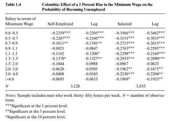
Another way to look at this data would be to examine the DiD effect sizes for wage changes as well as employment by the first wave wage variable. Overall, it can be seen that the magnitudes of the effect on wages and the effect on employment are positively correlated: the larger the wage change, the more negative the employment change. I think this study shows somewhat consistent proof that the minimum wage decreases employment, though, unfortunately, it is impossible to know if it is statistically significant.
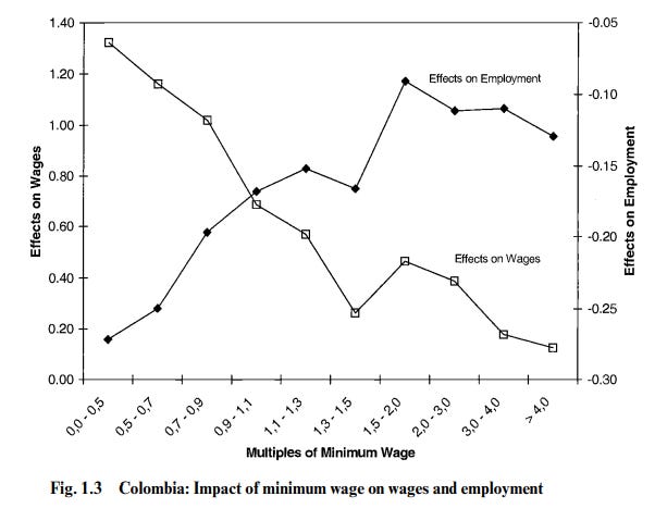
2.3.10. The 1987 Portugal Minimum Wage Spike
In 1987, two changes were made to the Portuguese minimum wage that greatly increased it for youths: The minimum for 17 year-olds became 75% of the adult minimum, whereas before it was 50%; in the same year, the minimum for those aged 18-19 became equal to the adult minimum, up from 75% of it. These changes correspond to increases of 50 and 33.33 percent, respectively. When Pedro Portugal and Ana Cardoso (2002) compared the employment growth of teenagers (17-19) to those somewhat older (aged 20-34), they found a statistically significant (p<0.05) positive effect. On the other hand, when they examined the share of new hires who were teenagers relative to those who were in the comparison group, the effect was negative and much more statistically significant (in the best model, from Table 5, column 4, p<0.0005). Similarly, the authors found that businesses that started after the minimum wage changes had a significantly lower portion of their employees be teenagers than businesses that began before the spikes. Also, teenagers were found to be overrepresented among firms shutting down, though this was only slightly significant in firms closing in 1988 and insignificant for ones closing in 1989. Lastly, they found that the treatment group was highly significantly more likely to be employed at the same firm after the increase than the control group. Overall, the results are mixed in terms of their direction, even though specific analyses often had statistically significant results.
As Neumark & Wascher (2006, pp. 103-104) pointed out, however, the figures regarding employment growth are based only on data from surviving firms, and no controls were used. These should be compared to the analysis provided by Pereira (2003), using essentially the same data (a 30% sample of it, rather than the full data used by Portugal & Cardoso). Using workers aged 20-25 and 30-35 as controls, she found that both groups’ employment increased relative to teenagers’ in the period following the spike, whether defined in terms of hours or employment rate, and whether the effect was measured across one year, two years, or three years. The more relevant comparison, the 20-25 year-olds, was significant at a p value below 0.01 in every specification. I think that the best available data show a decline in overall employment.
2.3.11. The 2019 Spain Minimum Wage Spike
In the beginning of 2019, the Spanish minimum wage was raised by over 20%. Pablo Laporta (2022) studied the effect of this increase on employment using a treatment group of those earning at or above the old minimum wage, but below the new minimum wage, in 2018. The control group is made up of those with wages at or up to thirty percent above the new minimum, with each member of the treatment group being compared to his closest match. The overall effect is an increase in the probability of job loss of 0.38 percentage points, or a relative increase in the probability of 7.8%, which effect is highly statistically significant (p<0.001; Table 1, column 4).
2.3.12. Trinidad and Tobago, 1998
In 1998, Trinidad and Tobago instituted a minimum wage which, for many occupations, was above the previous mean hourly wage! The effect of this increase was studied by Strobl & Walsh (2003), who used a basic longitudinal approach. The two variables which define the treatment group were the bound variable (i.e., dummy for earning less than the new minimum before it was instituted) and the wage gap variable. For men, both coefficients were large in magnitude (e.g., bound=1 indicated a 9% higher chance of losing your job), and were significant at the 10% and 5% levels, respectively. The effect sizes were much smaller for women and also nowhere near significance, but were still in the direction indicating negative employment effects. It should be noted that the authors found low compliance rates, which likely attenuated the effect toward zero.
2.3.13. The 1999, 2000, and 2001 U.K. Minimum Wage Spikes
in 1999, the U.K. reintroduced a national minimum wage after some time without one, and, in 2000 and 2001, this minimum was increased. The effects of all three increases were examined by Mark Stewart (2004), whose treatment group consisted of those earning below the new minimum, with a comparison group of those with wages equal to, and upwards of ten percent higher than, the new minimum. The results for all three increases varied between age and sex groups in terms of their direction, but none were anywhere near significance.
2.3.14. Summary
The table below summarizes the elasticity estimates I was able to find, though, unfortunately, there were not many:39

This method showed a much larger elasticity of -0.68, which was highly significant (p<1 × 10-19). It is not immediately obvious why the average effect here is much larger, but this arguably is the best measure, since it is not confounded by structural changes, and the fixed-effects model is much better at controlling for relevant variables than the typical set of covariates used in the other methods. When I asked ChatGPT to evaluate each method, giving it a basic explanation of each, and telling it to respond without consulting anything but its own logic, it agreed with me and ranked longitudinal studies above the other two methods, so this probably really is the best method. However, it is not clear if this could explain the entire difference.
3. Criticisms of the Time-Series Literature
Before the early 1990s, almost every analysis of the effect of the minimum wage on employment used what is known as the time-series method, in which, usually, the federal minimum wage in a given year was included in a regression on employment alongside basic variables like the seasonal variation in business cycles, time, and population share (since these were typically studies of teenagers, this variable would usually be equal to the percentage of the population made up of teenagers). In practice, the minimum wage variable (henceforth, MW) was almost always defined in terms similar to what I called bite in section 2.2. Most often, it was equal to the ratio between the nominal minimum wage and the mean wage, multiplied by the coverage rate. These studies, then, typically computed MW in a way that attempts to approximate change in wages as closely as possible—this is why I have been comparing these early time-series estimates, as summarized by Brown et al. (1982), to elasticities based on changes in average wages. Unfortunately, I am unaware of any study that looks at how well changes in the most common MW measure track onto changes in average wages.40
3.1. Publication Bias
This early time-series literature was criticized by Card (1995), who tested for publication bias in a meta-analytic sample of fifteen studies. He found that standard error was correlated positively with the magnitude of the elasticity estimate, and, more importantly, that studies tended to cluster around a t-ratio of 2.
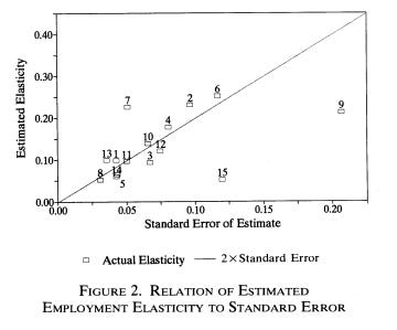
Card interpreted these results as showing publication bias because a t-value of 2 is roughly the threshold for significance (a t-value of 1.96 is p= ~0.05), and, if publication is largely contingent on permeating that threshold, t-values would converge at it. He theorized that this occurs specifically for two reasons: 1) the same specifications were used over and over if they had been proven to produce large elasticity estimates, and 2) research was simply not published when the authors fail to find significant findings. However, the pattern revealed in Card’s meta analysis does not look at all like what you’d expect from these effects!
Today, the causes proposed by Card would be separated into two categories (publication bias, and p-hacking, respectively), but, to be consistent, I will refer to both as publication bias. The effect of publication bias on the distribution of t-values in most lines of research can be exemplified by the following graph, from an analysis of the t-scores of about 1.3 million papers published in PubMed between 1976 and 2019 (Zwet & Cator, 2021).41

It can be seen that many t-values between -2 and 2 are “missing”. This is the obvious prediction of what publication bias would cause, since it is not being near the significance threshold that matters, but being past it. Clearly, the pattern observed in Card's data does not fit this at all, as, rather than being clustered above 2, the t-values were clustered on either side of it. This distribution can, in my opinion, be explained at least somewhat convincingly by the fact that there is a high degree of covariance across studies, as they all used similar methods, looked at similar time periods, and used essentially the same datasets. This covariance causes the ratio of the elasticity to the SE to be consistent across studies because the elasticity estimate and its standard error move in the same direction across studies. And, because the time-series method using national data is not a very powerful design (there are very few changes in the federal minimum wage, so most of the variation is caused by changes in coverage rate or median wages, leading to a lot of noise), the t-values would be likely to cluster around a small number—in this case, 2—because the signal to noise ratio is low.
Another explanation for this pattern was proposed by Neumark & Wascher (1998). They believe that Card’s finding could also be explained by changing parameters, meaning that the elasticity of labor with respect to MW changed over time. Using what they deemed to be the best specification in the literature, they find that the same pattern of t-values can be generated just by using the same specifications on different periods. Their distribution of t-values is actually much more indicative of publication bias than Card’s!
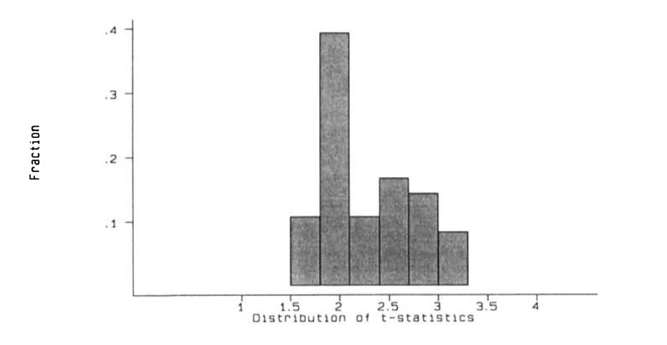
When they repeated the same analysis using a different, but very similar, model, they got results much closer to Card’s, and now no longer similar to what would be expected from publication bias.
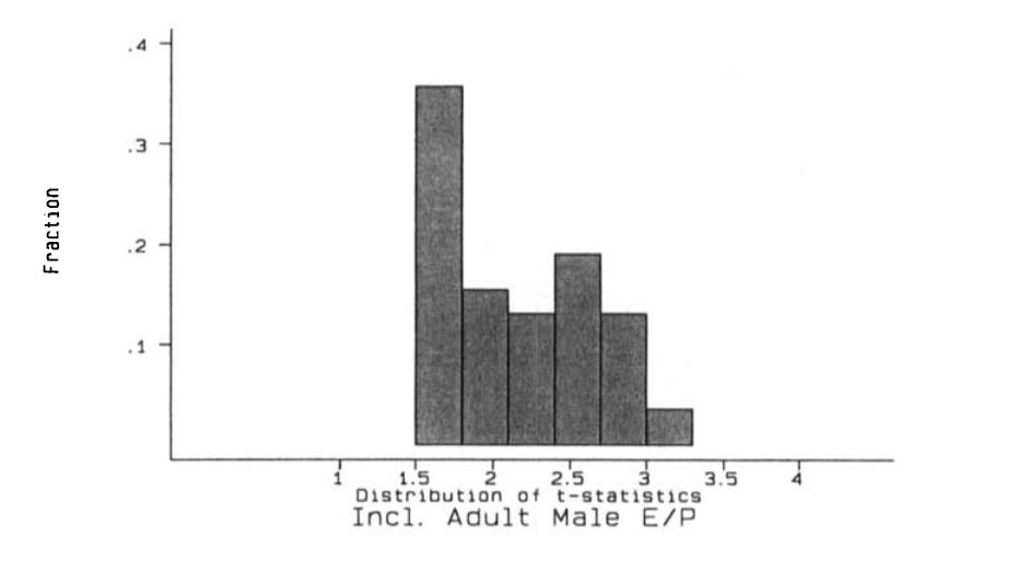
Because this pattern of t-values could be replicated by using one design—which, due to being different from the others in the literature, was deemed to be unlikely to have been chosen because of its likelihood to generate statistically significant results—and applying it to different years, Neumark & Wascher argued that this pattern could be caused by a decline in the true elasticity as the time-series expanded to include more years, while the SE decreased due to more observations adding more degrees of freedom. This argument is intuitively appealing because, unlike my explanation or Card’s, it reflects actual changes: decreasing effect sizes in the numerator, but also decreasing SEs in the denominator, both at a similar pace, leading to approximately constant t-values. However, there are two major problems with this explanation. The first is that it requires roughly proportional declines in standard error as in true elasticity, which would have to occur by chance,42 whereas the covariance hypothesis that I explained above would cause this pattern mechanically. The second problem, which is much less serious, is that two of the fifteen studies included in Card’s study began at a later year than the others (most began in 1954, but these at 1963),43 which would lead, according to Neumark & Wascher’s hypothesis, to a sharper decline in true elasticity than in standard error. This is because the decline in SE as the time-series includes later years is entirely based on the assumption that more year-quarter observations are included, or, put another way, that the time-series all start at the same year. Either way, it is clear that publication bias is neither the only nor the best explanation for this pattern.
3.2. The Method Itself
The main issue with the time-series method, according to Card & Krueger (1995, chapter 6), is that there is no control group: quarters with low MWs are compared to quarters with higher ones, but these are obviously not directly comparable, and the addition of various controls cannot definitively rule out all confounders. This is, of course, a sensible criticism, and few today would defend the method. Another unfortunate aspect of the time-series model is that, as seen above, most of the studies are done in basically the same way, using the same data, and covering the same time span, and so the method does not easily lend itself to pooled analyses such as those performed by me in section 2. Therefore, I am in agreement with the New Economics when it comes to the limited usefulness of the method, as are, I think, most traditional economists.
3.3 Time-Series Using State-Level Variation
Some studies have used a state-level version of the time-series approach, though these were not published until the 1990s, as before then there was too little variation in states’ nominal minima. These studies are far superior to the traditional method because they allow better controls and have more power. The first such study was published by Neumark & Wascher (1992), who used a state-level version of the most common MW, and found results similar to the national-level literature. However, their paper was soon criticized by Card et al. (1994), who pointed out that their main model included a covariate representing state-level school enrollment rate, which actually only included those who were enrolled and not working. This meant that Neumark & Wascher had accidentally partially controlled for the dependent variable in their regression, which, because it is negatively and mechanically correlated with employment, may have exaggerated the coefficient of MW. To demonstrate this empirically, Card et al. used the same enrollment variable, but estimate enrollment and employment using data that overlaps very little. This led the enrollment variable’s coefficient to shrink to a fifth of its size, suggesting that most of its effect had been caused by mechanical bias.
Finally, they also pointed out that the MW variable used by Neumark & Wascher was negatively correlated with teenage wages, whereas nominal minimum wage was very highly correlated with wages. Therefore, they argued, their index did not properly measure the minimum wage. Of the two major flaws that they point out, this one is by far the weaker one. There are many reasons that the MW index would be negatively correlated with state-level wages, especially since adult wages were controlled for (as Card et al. noted), and since, at any given nominal minimum wage, the MW index decreases as median wages increase by construction! The MW variable represents, roughly, how much wages are being pushed up by the legal minimum, and is therefore not necessarily supposed to correlate positively with wages. On top of this, though, Card et al. do provide a more serious reason for concern, namely, that coverage was based on the portion of the state’s working age population which was covered by the federal minimum wage, and was therefore not directly applicable to either teenagers specifically or to state-level minima. Unfortunately, no alternative measure of coverage had been published up to that point.
In response, Neumark & Wascher (1994) saw whether an alternative enrollment variable that more accurately represented the proportion of youths attending school—more specifically, the variable was equal to the portion of youths reporting that attending school was their primary activity—obtained different results. In fact, their results did not differ much between specifications: using the original enrollment variable, the elasticities were -0.19 for teens (16-19) and -0.17 for youths generally (16-24), and, using the alternative, these were -0.11 and -0.16, respectively. In both cases the difference between the results was insignificant, though, in the case of teens, the elasticity estimate stopped being significant when the alternative variable was used (the other three elasticities were significant).
Next, they responded to the criticisms pertaining to the coverage variable by rearranging their equation such that coverage is added as a covariate and the MW variable is changed into just the median wage to nominal minimum wage ratio. They find that the coverage variable itself also negatively correlates with employment, and that the new MW variable is still negatively correlated with it, too. Because coverage has its own independent effect, Neumark & Wascher argue that it likely is measuring what it is intended to. Furthermore, they also noted, as I did, that it is wrong to conclude that a negative correlation between MW and wages is unexpected. Using a different approach, they found that MW is positively correlated with the ratio of teen wages to overall mean wages, which matches theoretical expectations.
I believe that Neumark & Wascher ended up winning this debate, though both national and state-level time-series studies almost completely died out by 2000, and a detailed analysis of the modern literature would probably be a waste of time. Still, my impression, primarily based on some of the discussions in the studies I read while writing this post, is that an elasticity around -0.1 to -0.2 has held up.
3.4. Summary
The time-series method was, I think, inappropriately maligned by Card, as well as by the New Economics in general. There is very little evidence that publication bias played a large role in shaping its derived elasticities, and the classical range of -0.1 to -0.3, or perhaps -0.1 to -0.2 in the best studies, is not very far off from what is suggested by the methods promoted in the New Economics. That being said, though, moving away from it and toward more direct models will probably prove beneficial for the field in the long term, especially if more researchers begin to notice that these newer methods come to the same conclusion when pooled together: a sizeable negative elasticity.
4. Recent Literature Reviews
In this section, I discuss recent reviews (i.e., those published in 2019 or later). As a rule, I decided that I would not include any of the studies mentioned in these reviews if I had not already included it in section 2—which I finished writing shortly before moving onto this section—unless it was a replication of a study which I did include, I noticed that there were many high-powered studies that found results inconsistent with my own (i.e., elasticities significantly above or below -0.2). This was mostly done in order to publish this article sooner, and none of the exceptions ended up applying.
4.1. Dube (2019)
Before beginning this section, I must note that there are two types of elasticities in this literature—those where change in employment is divided by the change in the nominal minimum wage (MWE, minimum wage elasticity), and those where change in employment is divided by the change in wages (OWE, own-wage elasticity). Throughout this review, I have used the latter equation, but the former is much more common in the literature. The issue with the more common measure is obvious, namely, that the medium through which the minimum wage must affect employment must be wage increases. This was emphasized by Dube in his review:
[T]he MWE is not a particularly useful way of summarizing the impact of minimum wages when comparing across groups and minimum wage experiments with very different “bite” of the policy. For example, consider case A, where a minimum wage increase that is binding for 10% of the workers overall, 15% of those in retail, and 40% of those in restaurants, versus case B, where it’s binding for 5% overall, 10% in retail and 30% of those in restaurants. Study # 1 may use case A, and report the estimate for restaurants (40% bound), while another study # 2 may use case B and retail (10% bound). The bite of the policy is quite different across the two studies because in general case study # 1 is using a more generally binding minimum wage increase, and because it is using a generally lowerwage group. A more useful measure that accounts for these discrepancies is the “own-wage employment elasticity” (OWE), which tells us how employment for the specific group responds to an increase in the average wage of that group induced by the minimum wage change. (p. 26)
His conclusion, based on an analysis of 55 studies, was that the OWE is, on average, -0.17 for “any group” and -0.04 for “overall low wage workers”. This is not weighted by standard error or any other variable. The -0.17 figure essentially matches my findings, and, given that it represents all of the data rather than just a small subset, it is probably the best figure one can get from Dube’s report.
4.2. Wolfson & Belmen (2019)
These authors conducted a meta-analysis of studies published since the end of 2000. They found 60 studies, of which 37 allowed a calculate of an MWE. Overall, they found a mean elasticity of -0.063 using all estimates, and a median of -0.03. The authors concluded that there was little evidence of publication bias based on the distribution of elasticities. When using only one estimate per study—considered to be the best estimate from each—the mean and median become -0.16 and -0.08, though publication bias becomes much more apparent (with a bias toward more negative estimates). Finally, when each study’s estimates were averaged out, and then those averages were used in the calculations, the mean became -0.09, and the median, -0.05.
When the elasticities were weighted by standard error, the analysis that included all estimates from each study separately showed a mean of -0.024, while the same figures for the other two types of analyses were -0.115 and -0.12 (one effect per study and each study’s average only, respectively). When the authors adjusted their results for publication bias, and included other important variables like dummies for which study the effect sizes came from, they found a statistically significant MWE of -0.11 on teenage employment (p<0.05).
4.3. Campolieti (2020)
Campolieti published a meta-analysis of Canadian studies. In her search of several databases, she discovered 49 studies, of which sixteen were included in the analysis. From these studies, she was able to extract hundreds of individual estimates. In the main table (Table 3), the estimated effect on employment, weighted for standard error, was negative, but only became statistically significant after restricting the sample to seven studies that used the same measure of employment. For teenagers, the effect was an MWE of -0.321, and, for all youths, -0.225. These had p values of less than 1 × 10⁻⁸ and 5 × 10⁻⁶, respectively. When Campolieti allowed only one estimate per study, she got similar point-estimates (-0.278 and -0.231 for teenagers and all youths, respectively), but these were less significant (ps= ~0.018 and ~0.0054). In these regressions, the estimated effect of publication bias was smaller and remained insignificant.
4.4. Neumark & Shirley (2022)
These authors reviewed 70 papers published since 1992 which analyzed U.S. data. Rather than a typical meta-analytic approach, the authors only took the authors’ best estimates for each study, determined through reading the text and emailing the authors. They found that 79.2% of the elasticities were negative, and 46.2% were both negative and statistically significant. On the other hand, less than 21% were positive, and only 3.8% were statistically significant in the positive direction.
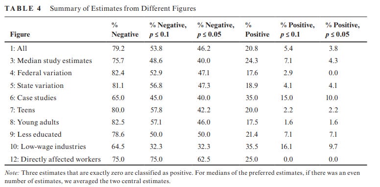
The overall mean elasticity was -0.15, while the median was -0.12. If instead of taking all of the preferred estimates from each study, each study was assigned the value of its median preferred estimates, the mean and median remained similar: -0.13 and -0.11, respectively. Unfortunately, weighted summary statistics are never provided. Also, the elasticities are not necessarily comparable, mostly because some are MWEs while others are OWEs.
4.5. Dube & Ziperrer (2024)
In this meta-analysis, 88 studies were included, and they presented the OWEs for each. By my count, there were 11 statistically significant negative effect sizes and only two statistically significant positive ones (based on Figure 2, ignoring studies without CIs). The mean OWE was -0.22 among all studies, while the median was only -0.14. However, because these figures are unweighted, they do not necessarily indicate skew in the normal sense of the term, as each point-estimate is extremely imprecise. Still, both are essentially in line with my findings above, with OWEs slightly below -0.2. When weighted for precision, however, the median became zero and the mean, -0.1—quite a remarkable finding, which, for some reason, was not mentioned at all in the main text (but, rather, only in Table 3).
Because this is the most recent review, it is worth comparing its treatment of studies to mine. Of the 72 studies included in their review, only 10 were also included in my final analysis. However, this lack of overlap is largely caused by the fact that I only used one estimate per case per method whenever possible, and because I used replications whenever possible. Furthermore, many of the papers in their review would not fit my criteria (e.g., time-series studies). By my count, 27 of their 72 papers were either cited here or otherwise recognized by me as ones that I had looked at during the time that I spent writing this article, and I think a reasonable estimate would be that I included about 2/3 of the relevant studies which also appeared in Dube’s article (i.e., excluding studies that don’t fall into any of the three methods I focused on). The table below summarizes the conclusions of both mine and their review about each study we shared in common:44
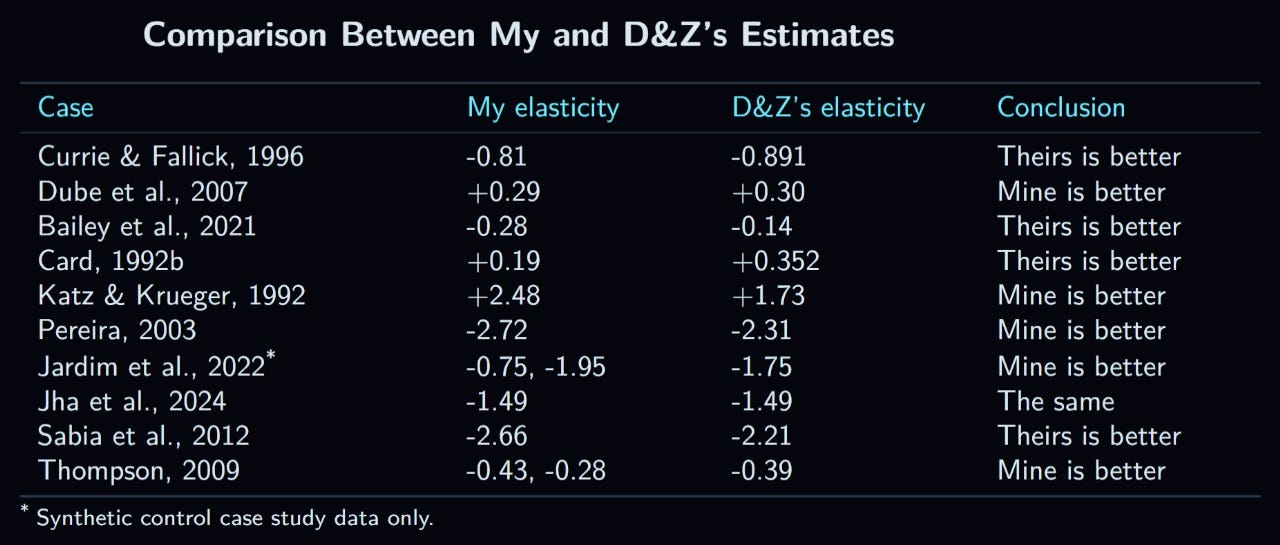
It can be seen that, in most cases, our estimates were very similar, but, only in one case, actually the same. Typically, the differences were caused by choosing different specifications or choosing different groups for analysis (e.g., if results for 16-19 year-olds and 20-24 year-olds are given separately). These are mostly matters of opinion, and so I will not focus on them here; for a discussion of each of these studies separately, see Appendix A for this post. Of more immediate interest are the few cases in which I think actual mistakes were made; there were three instances of this, all of which were my own:
For Currie & Fallick (1996), I did not divide the employment change by the baseline employment change, which was available. This meant that the numerator of my elasticity estimate was something other than a percent change, while the denominator was percent change. This makes very little difference in real terms, however.
When analyzing Card (1992b), I made the same mistake of not dividing by the baseline proportion, and this time it made a very big difference. However, note that when scaling the elasticity, the SE is scaled to the same extent, which means that even this quite large mistake would have very little impact on the weighted elasticity.
And, lastly, when looking at Sabia et al. (2012), I used log income change in the denominator rather than percent change, which was what I used in the numerator. This mistake made basically no difference.
On top of correcting my two mistakes, I also agreed with Dube & Zipperrer in a few cases on, for example, which column of a table they chose. After revising all of the estimates (not shown in the table), my unweighted average elasticity for these 10 studies decreased from -0.7 to -0.64. Note that I did not update my results, as finding the exact answer is not the goal—being approximately correct is good enough. The point of the present discussion is only to see if I am very far from being correct, and I don’t think that this small difference is indicative of that. I conclude that my numbers are probably okay, though of course imperfect, as shown by the few silly, but not meaningful, mistakes that I caught by comparing my estimates to Dube & Zipperrer’s.
5. Does the Economy Benefit?
In this section, I aim to answer perhaps the most important question: Overall, does the economy benefit from raising the minimum wage? First, I look at the elasticity of price to see how minimum wage increases affect the cost of goods, focusing almost entirely on the fast food industry. In the next section, I examine the effect on business profits. The third section is a crude cost-benefit analysis for the fast food industry as a whole.
5.1. Price
The fact that prices rise with increases in the minimum wage is much less contentious in the minimum wage literature, and is accepted in the New Economics, though there is no standard elasticity estimate for price. In order to estimate how large this effect is, I tried to find every study included in section 2 which had wage data, price data, and the possibility of calculating the standard error.45 Whenever possible, I focused specifically on fast-food wages and prices. The table below summarizes the results of my effort:
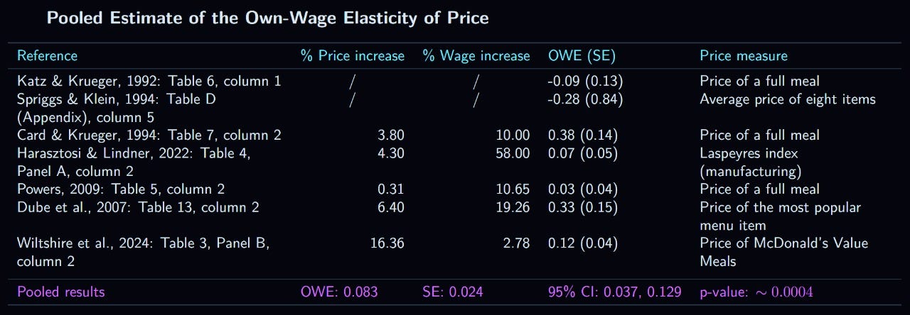
The average OWE for price was a little over 0.08, meaning that raising the minimum wage such that wages increase by 1% also increases the price (typically of meals at fast food restaurants) by 0.08%. However, the confidence interval for this estimate is much wider than for the employment data, and so it should be interpreted cautiously.
5.2. Profits
The evidence regarding profits is much scarcer. As far as I remember, only one study in my review directly examined this, and it found a highly statistically significant negative effect (p<0.0005; Harasztosi & Lindner, 2022, Table 3, column 1). Another paper, not included in this review,46 also found a highly significant negative effect on business profits (p<5 × 10-24; Drucker et al., 2021, Table 5, column 3). These two studies on their own, I think, are enough to conclude that the effect on profits is negative, despite businesses’ attempt to cut back the losses by reducing the number of workers and by raising prices. The OWE of price, based on the first study, is -0.59, with an extremely tight 95% CI ranging from -0.6 to -0.58.47
5.3. The Answer
Here, I simplify the entire low-wage economy to consist of three groups, businesses, consumers, and low-wage workers. Owners of businesses that employ workers at low wages are affected by changes in profits; consumers of goods and services produced in low-wage industries are affected by changes in price; and those employed at low wages are affected by changes in wages and employment. For workers, the effect is not all that controversial: of course, they benefit, because their wages go up. This is slightly offset by decreasing employment, but assuming a perfectly linear labor elasticity (i.e., employment decline is always at x% of the level of minimum wage increase), the net wage effect does not turn negative until the increases reach around 400%!48 But, despite the wage effect certainly being positive, one must weigh it against the effect on profits and prices. A minimum wage spike that would increase income of low-wage workers (contingent on employment) by 10% would increase overall wages by 7.47% for that group of workers (i.e., after setting the incomes of those who lose their jobs to zero), increase prices by 0.83%, and decrease business profits by 5.90%.
In order to conduct a cost-benefit analysis, I used U.S. data for the Fast food industry, as provided in a 2010 IBISWorld report. In that year, overall profit for the fast food industry was $8.3B, total wage costs were $48B, and sales were $184B. According to ChatGPT, the wages figure should be multiplied by 0.65, as about 15% of all wages typically go to higher paid supervisory workers, and some of the wage expenses are in non-monetary benefits. The wage figure, then, becomes approximately $31B.
The following table offers a crude estimate for how a 10% spike in nonsupervisory fast food workers’ wages would effect the industry in dollar terms:
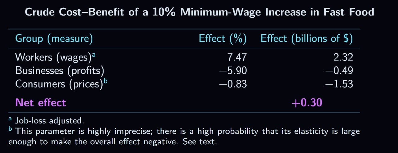
It can be seen that the effect is positive—unexpected, to be honest. However, this estimate is not very precise. If the upper bound of the confidence interval reported in section 5.1 is used, then the overall effect becomes -$0.55B. Indeed, the probability that the true price OWE is high enough to make the estimate neutral or negative, based on my pooled sample, is almost one in four.49 Perhaps, in the future, I will attempt a more complete analysis of the price elasticity, and repeat these estimates.
6. Summary & Conclusion
The summary section comes first. In it, I discuss my results in section 2 as well as my summary of recent meta-analyses in section 4. In the next section, I present my conclusions.
6.1. Summary
Despite many claims that the minimum wage does not decrease employment—mostly made by advocates, but also sometimes by serious researchers like David Card and Alan Krueger—every form of evidence examined here has shown that it does. The reason that such a conclusion could have been reached in the first place, aside, of course, from political bias, is that the main method promoted in the New Economics literature (case studies) is extremely noisy. As shown in section 2.1d, not a single one of over two dozen case studies had enough power to detect an elasticity of -0.2 eighty percent of the time, with the average power being just 13%, and the median only 12%.
The table below summarizes all of the studies reviewed here, irrespective of whether or not they supplied enough information to calculate an elasticity and standard error, and including some duplicates.
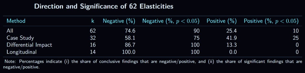
Overall, about three fourths of non-inconclusive estimates were in the negative direction, and, of statistically significant findings, 90% were negative. These findings roughly match the table provided by Neumark & Shirley (2022), shown above, which was my stylistic inspiration. Next, here are the meta-analytic results:

The weighted mean is -0.23, matching the classical estimate around -0.2 quite well. The longitudinal data are an outlier, which, as I wrote earlier, may be partially explained by the fact that it is a better method, and so catches more of the effect. Other recent literature reviews (discussed in section 4) have found OWEs around -0.2 and MWEs ranging from roughly -0.1 to -0.3. These results are similar to mine (an OWE of -0.2), but it should be noted that the two OWE results are unweighted, and that MWEs are not directly comparable to OWEs. Most noteworthy is the fact that all of the recent reviews I could find concluded that the elasticity was significantly negative.
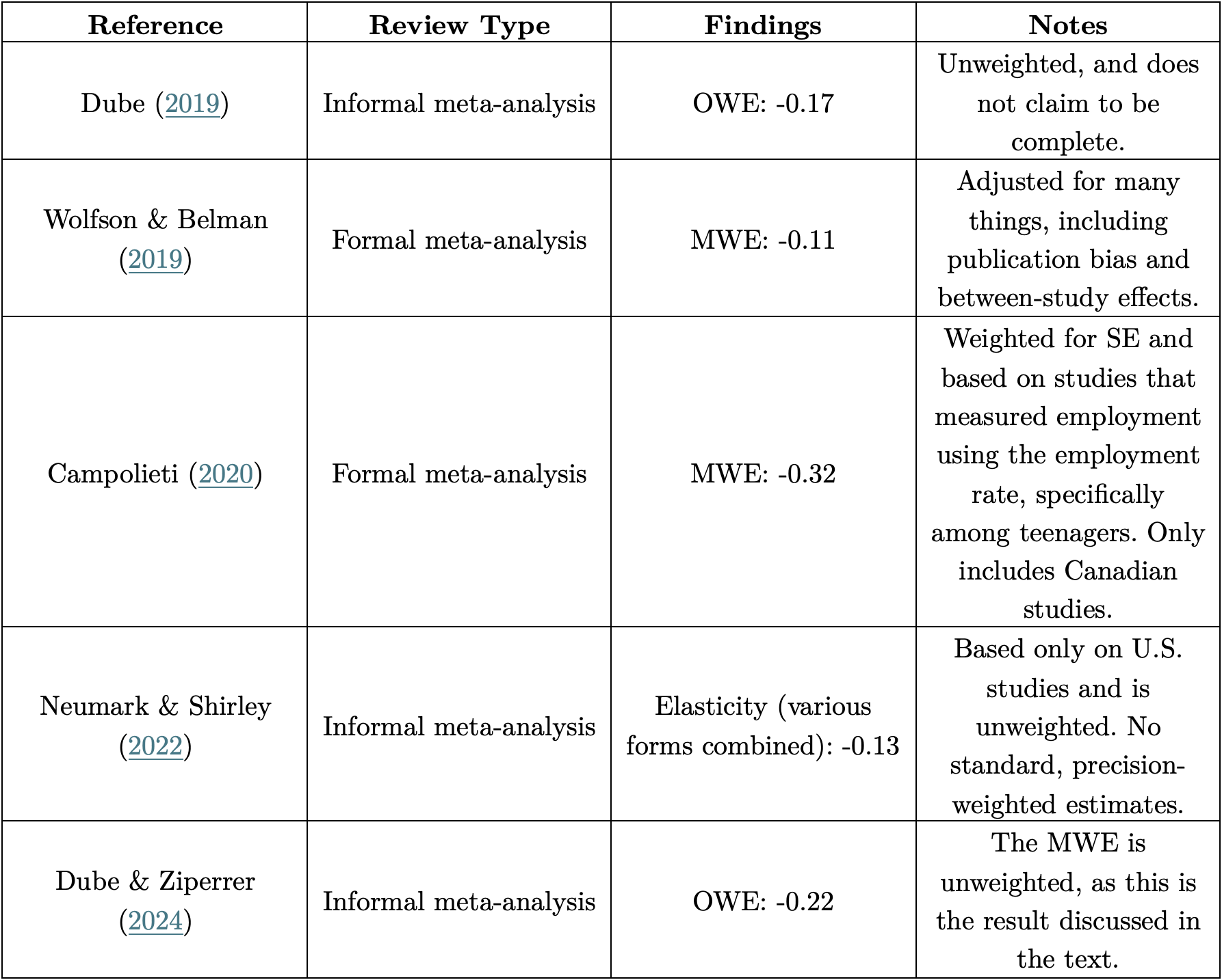
6.2. Conclusion
The theoretical evidence in favor of the minimum wage reducing employment is extremely strong. Simply put, the elasticity of demand for everything else is negative, so why wouldn’t that also be the case for labor? By the early 1980s, Brown et al. (1982) concluded their famous report by arguing for an elasticity of labor of -0.1 to -0.3 based on the time-series literature. However, about a decade later, several researchers—most notably, David Card and Alan Krueger—began to argue that better methods reach a different conclusion: an elasticity of approximately zero. This line of research is what I continually referred to as the New Economics.
However, these researchers were wrong. Their methods were too noisy to form conclusions based off of just a few early studies. To this day, the most popular method, the case study approach, has never produced a single study with enough power to consistently detect an elasticity of -0.2; not even close. The two other methods promoted by the New Economics are not as noisy, but only three studies using these methods were available to Card & Krueger when they wrote the book which defined the field, Myth and Measurement (1995). In an informal meta-analysis, I found an overall elasticity of -0.23, in line with the classical consensus reached more than forty years ago. Similar estimates have come from the most recent meta-analyses.
Furthermore, I also prevent evidence that the OWE of price is around 0.1, and that the OWE of profit is about -0.6. This means that any serious discussion about the benefits of the minimum wage must also address its effects on price and business profits. My own cost-benefit analysis found that a 10% increase in fast food workers’ wages would have a positive impact of a little under $300M, but this effect is highly dependent on an imprecisely measured parameter (OWE of price), which has an almost 24% chance of being large enough to make the overall impact negative.
To conclude, the elasticity of labor is definitely negative, but not so negative that the overall net effect on workers is negative when the wages of those who lose their jobs are set to zero. Furthermore, the minimum wage also certainly increases the price of goods produced in low wage industries, and also reduces business profits. However, it is difficult to construct a precise cost-benefit analysis, as the change in price has a wide confidence interval. Thus—employment and profits definitely go down, and price certainly increases, but nobody knows what happens on balance. Claims that there are essentially no detrimental effects of minimum wage increases, made by some advocates like Robert Reich, are obviously insane; but almost as crazy are claims made by some advocates on the other side; just yesterday, the Libertarian Party’s official X/Twitter account posted a video saying that the effects of a minimum wage increase is “apocalyptic”, which Matt Darling rightfully derided, saying, “If a policy has ‘apocalyptic’ results it shouldn’t really matter exactly how you are measuring employment levels across state lines”.50
Appendix A: Comparison with Dube & Zipperer’s Meta-Analysis
Here, I elaborate on the differences between mine and Dube & Zipperrer’s (2024; henceforth, D&Z) elasticity estimates from the ten studies we shared in common.
Note: all of the decisions made by D&Z were in pursuit of selecting the authors’ preferred estimate from each study, sometimes through direct communication, so the decisions were not necessarily their own. Furthermore, their design was such that only one estimate was allowed per study, so in a few cases they summarize a study of multiple spikes with just one estimate.
1. Currie & Fallick (1996). D&Z divided the absolute effect by the baseline probability of attrition, to turn it into a relative change, which I neglected to do. This is important because elasticity is calculated in terms of (change in employment)/(change in wages), but does not matter very much, as the divisor is 0.97. They also used a different specification for increase in employment, namely, Table 2 column 4, rather than column 5, which I used. In the fifth column, a control is added for being near the minimum. This control is arguably important because the effect of being affected by the increase might be confounded by the effect of simply having a low wage. However, because this variable has an effect size of essentially zero and is not significant, and also does not change the coefficient of the gap variable to any significant degree, including it might not be very wise. This decision is also probably in their favor, though it again changes little. We calculated change in the mean wage in the same way. In conclusion, the best estimate is exactly theirs, at -0.891.
2. San Francisco (2004). Our calculations for change in wages were the same, but we differed slightly when it came to calculating changes in employment. While I used changes in full time equivalent employment, they used changes in employment rate. This did not result in a very large difference, but mine is better, as employment in economic terms is shorthand for time worked, or some other similar version of “work done” that is better measured in FTE workers than overall employment.
3. Card (1992b). Here, I differed slightly from D&Z in that I used the coefficient given in Table 4, row 6, column 7, while they used row 6, column 5 of the same table. For the same reason given in the first section of this Appendix, I concur that their specification is the best, as the one I used has the same explanatory power, and therefore the added control is not useful. However, this difference only explains a very small portion of the disagreement between our estimates. What causes most of this difference is D&Z’s correct decision to divide the elasticity estimate by 0.445, i.e., the baseline employment rate. As explained earlier, this is necessary, and, unfortunately, makes a large difference.
4. Katz & Krueger (1992). I used the same table as D&B, but, while they looked at overall employment rate, I used FTE employment. I believe that the figure I used was the correct one, for the reason given above.
5. Portugal (1987). Our analyses differed in two ways: 1) I used data for 20-25 year-olds, while they used the results for 30-35 year-olds; and 2) they used overall employment rate while I used hours worked. I believe that my decision in both instances was the better one.
6. Bailey et al. (2021). We both used Table 3, but I used a different dependent variable—hours worked rather than the proportion employed during the last year—and also a different specification (column 4 instead of 3). I believe that hours is the superior choice, but that D&Z’s chosen specification was better. This is because the specification I used adds controls for states’ average gross product, which is hard to justify when their model already includes state-cohort fixed effects. Their figure is closer to the best one, but my overall pick would be -0.07 (Table 3, column 3).
7. Jardim et al. (2022). We used the same wage estimates from Table 6A, but, whereas D&Z used the jobs data (Table 6C), I used the hours data (Table 6B). I believe that my choice is better for reasons specified earlier. Furthermore, we also differed in that they computed only one estimate, whereas I computed two—one for each of the two spikes that occurred in the period. And, lastly, while I used three quarters of data for each spike, they simply used the last quarter, 2016:III. This is probably not a terrible choice on their part, since the latest quarter reflects the cumulative changes, but I think that my approach is still better in practice, since much of the between-quarter variance is caused by random error. Furthermore, it is not certain that the third quarter of 2016 captures the effect better than, say, the first quarter, even though this likely is the case. For these reasons, I think my estimate is better.
8. Jha et al. (2024). We both used the same specification (Table 3, column 1) and came up with the same elasticity.
9. Sabia et al. (2012). D&Z’s estimate comes from the elasticity estimates provided by the authors, which are in the form of MWE. Simply, they divide the MWE for employment (Table 3, column 5) by the MWE of wages (Table 2, column 5). My approach was very similar, except for the fact that I analyzed 16-19 year-olds specifically, rather than the full youth sample, and except for the fact that I calculated the elasticity manually using the more specific numbers they provided. I made two mistakes in my analysis: 1) I used column 6 of table 3 to calculate employment change, whereas column 5 is preferred due to being consistent with where I am getting my wage estimate from (table 2 did not have a sixth column; the sixth column adds certain controls which, arguably, are not necessary in the first place, and are especially a problem because no comparable estimate for wages is given); and 2) I left the log change in minimum wage in the denominator instead of turning it into a percent change. If done correctly, my estimate changes to -2.25, which is almost the same as D&Z’s estimate (remember that I only use teenagers in my estimate rather than the entire youth sample). Overall, theirs was certainly a better estimate than my original, but the best estimate is -2.25, as I think that teenagers are a better group to use for this analysis.
10. Thompson (2009). As described in the text, this author used three different bite measures. I believe that the continuous measure is clearly the best, while D&Z use the “thirds” measure, in which counties in the bottom third of the teen income distribution are compared to counties in the top third of the same variable. Furthermore, Thompson studied two different federal minimum wage spikes, but D&Z only examine data for the first. I think that both differences are in my favor, but the results are essentially the same—their estimate for the 1996 spike is -0.39, whereas mine is -0.43.
Appendix B: Recommendations for Further Learning
Here, I suggest what to read and watch for those who want to learn more about the empirical literature surrounding the minimum wage.
What to Watch
While researching for and writing this article, I listened to three talks:
David Neumark: “Using Minimum Wages to Fight Inequality and Poverty” (UCI, not dated);
David Neumark: “What Can We Conclude from the Evidence on Minimum Wages and Employment? Recent Progress” (Hoover Institute, 2022); and
Alan Krueger: “Plenary Session: Minimum Wages” (Royal Economic Society, 2015)
I would recommend listening to the first talk by Neumark if you care about how successful (or unsuccessful) the minimum wage is at reducing poverty—he has many interesting things to say. The second Neumark talk is more focused on the technical aspects of the literature, so whether or not you should listen to it depends on how serious you are about the topic. Alan Krueger’s talk is a good summary of his and Card’s 1995 book, and of the position of the New Economics generally, so it is a great substitute for reading their book if you don’t have the time to, but still want to hear both sides of the issue. It also features brief talks from a few other prominent New Economics figures, such as Dube.
What to Read
The best book I was able to find was David Neumark and William Wascher’s, published in 2008, which I have cited throughout the text. Card and Krueger’s is a good summary of the views of the New Economics, and also a good summary of all of Card and Krueger’s studies on the minimum wage. Unfortunately, I did not have time to read the 20th anniversary edition of that book, nor did I read another very important book published around the same time, titled, What Does the Minimum Wage Do? (Belman & Wolfson, 2014). Therefore, I cannot say whether these books are good or not, but you should probably read them anyway if you have the time; I just couldn’t justify it because, as I am writing now, I have been working for almost two months on this article, and don’t care to spend any more time than I need to.
References
Ahlfeldt, G., Roth, D., Seidel, T. (2018). The regional effects of Germany’s national minimum wage. Economic Letters, 172, 127-130.
Alatas, V. & Cameron, L. (2003). The impact of minimum wages on employment in a low income country : an evaluation using the difference-differences approach (English). World Bank Group: Research working paper series, No. WPS 2985.
Albinowski, M. & Lewandowski, P. (2022). The heterogeneous regional effects of minimum wages in Poland. Economics of Transition and Institutional Change, 30(2), 237-267.
Allegretto, S., Godoey, A., Nadler, C., & Reich., M. (2018). The New Wave of Local Minimum Wage Policies: Evidence from Six Cities. Report published by the Center of Wage and Employment Dynamics.
Andreyeva, T., Long, M., & Brownell, K. (2010). The Impact of Food Prices on Consumption: A Systematic Review of Research on the Price Elasticity of Demand for Food. American Journal of Public Health, 100(2), 216-222.
Arnadillo, J., Fuenmayor, A., & Granell, R. (2024). The relationship between minimum wage and employment. A synthetic control method approach. The Economics and Labor Relations Review, 35(3), 771-791.
Ashenfelter, O. & Card, D. (1981). Using Longitudinal Data to Estimate the Employment Effects of the Minimum Wage. London School of Economics, Discussion paper, No. 98.
Baek, J. & Park, W. (2016). Minimum wage introduction and employment: Evidence from South Korea. Economics Letters, 139, 18-21.
Bailey, M., DiNardo, J., & Stuart, B. (2021). The Economic Impact of a High National Minimum Wage: Evidence from the 1966 Fair Labor Standards Act. Journal of Labor Economics, 39(2), 329-367.
Bazen, S. & Skourias, N. (1997). Is there a negative effect of minimum wages on youth employment in France? European Economic Review, 41(3-5), 723-732.
Beauchamp, A. & Chan, S. (2014). The Minimum Wage and Crime. The BE Journal of Economic Analysis & Policy, 14(3), 1213-1235.
Belman, D. & Wolfson, P. (2014). What Does the Minimum Wage Do? Upjohn Press.
Bhorat, H., Kanbur, R., & Stanwix, B. (2014). Estimating the Impact of Minimum Wages on Employment, Wages, and Non-Wage Benefits: The Case of Agriculture in South Africa. American Journal of Agricultural Economics, 96(5), 1402-1419.
Bossler, M., Chittka, L., & Schank, T. (2024). A 22 Percent Increase in the German Minimum Wage: Nothing Crazy! IZA Discussion Paper, No. 17575.
Brown, C., Gilroy, C., & Kohen, A. (1982). The Effect of The Minimum Wage on Employment and Unemployment. Journal of Economic Literature, 20(2), 487-528.
Bruttel, O. (2019). The effects of the new statutory minimum wage in Germany: a first assessment of the evidence. Journal of Labour Market Research, 53: 10.
Caliendo, M., Fedorets, A., Preuss, M., Schröder, C., & Wittbrodt, L. (2018). The short-run employment effects of the German minimum wage reform. Labour Economics, 53, 46-62.
Campolieti, M. (2020). Does an Increase in the Minimum Wage Decrease Employment? A Meta-Analysis of Canadian Studies. Canadian Public Policy, 46(4), 531-564.
Card, D. (1992a). Do Minimum Wages Reduce Employment? A Case Study of California, 1987–89. ILR Review, 46(1), 38-54.
Card, D. (1992b). Using Regional Variation in Wages to Measure the Effects of the Federal Minimum Wage. ILR Review, 46(1), 22-37.
Card, D. (1995). Time-Series Minimum-Wage Studies: A Meta-analysis. The American Economic Review, 85(2), 238-243.
Card, D., Katz, L., & Krueger, A. (1994). Comment on David Neumark and William Wascher, “Employment Effects of Minimum and Subminimum Wages: Panel Data on State Minimum Wage Laws”. ILR Review, 47(3), 487-497.
Card, D. & Krueger, A. (1994). Minimum Wages and Employment: A Case Study of the Fast-Food Industry in New Jersey and Pennsylvania. American Economic Review, 84(4), 772-793.
Card, D. & Krueger, A. (1995). Myth and Measurement: The New Economics of the Minimum Wage. Princeton University Press.
Card, D. & Krueger, A. (2000). Minimum Wages and Employment: A Case Study of the Fast-Food Industry in New Jersey and Pennsylvania: Reply. American Economic Review, 90(5), 1397-1420.
Cengiz, D., Dube, A., Lindner, A., & Zipperer, B. (2019). The Effect of Minimum Wages on Low-Wage Jobs. The Quarterly Journal of Economics, 134(3), 1405-1454.
Clemens, J. & Wither, M. (2019). The minimum wage and the Great Recession: Evidence of effects on the employment and income trajectories of low-skilled workers. Journal of Public Economics, 170, 53-67.
Clemens, J., Edwards, O., & Meer, J. (2025). Did California’s Fast Food Minimum Wage Reduce Employment? NBER Working Paper, No. 34033.
Currie, J. & Fallick, B. (1996). The Minimum Wage and the Employment of Youth Evidence from the NLSY. The Journal of Human Resources, 31(2), 404-428.
Datta, N. & Machin, S. (2024). Government contracting and living wages > minimum wages. CEP Discussion Papers.
Dolado, J., Kramarz, F., Machlin, S., Manning, A., Margolis, D., & Teulings, C. (1996). The economic impact of minimum wages in Europe. Economic Policy, 11(23), 317-372.
Drucker, L., Mazirov, K., & Neumark, D. (2021). Who pays for and who benefits from minimum wage increases? Evidence from Israeli tax data on business owners and workers. Journal of Public Economics, 199, 104423.
Dube, A., Naidu, S., & Reich, M. (2007). The Economic Effects of a Citywide Minimum Wage. ILR Review, 60(4), 522-543.
Dube, A., Lester, W., & Reich, M. (2010). MINIMUM WAGE EFFECTS ACROSS STATE BORDERS: ESTIMATES USING CONTIGUOUS COUNTIES. The Review of Economics and Statistics, 92(4), 945-964.
Dube, A. & Zipperer, B. (2015). Pooling Multiple Case Studies Using Synthetic Controls: An Application to Minimum Wage Policies. IZA Discussion Paper, No. 8944.
Dube, A. (2019). Impacts of Minimum Wages: Review of the International Evidence. Independent Report Published by the U.K. Government.
Dube, A. & Ziperrer, B. (2024). Own-Wage Elasticity: Quantifying the Impact of Minimum Wages on Employment. NBER Working Paper, No. 32925.
Fone, Z., Sabia, J., & Cesur, R. (2023). The unintended effects of minimum wage increases on crime. Journal of Public Economics, 219, 104780.
Garloff, A. (2017). Side effects of the introduction of the German minimum wage on employment and unemployment: Evidence from regional data – Update. Bundeswirtschaftsministerium für Wirtschaft und Energie, Diskussionspapier, Nr. 4.
Gindling, T. & Terrell, K. (2007). The effects of multiple minimum wages throughout the labor market: The case of Costa Rica. Labour Economics, 14(3), 485-511.
Giupponi, G., Joyce, R., Lindner, A., Waters, T., Wernham, T., & Xu, X. (2024). The Employment and Distributional Impacts of Nationwide Minimum Wage Changes. Journal of Labor Economics, 42(1), 293-333.
Hakobyan, S. (n.d). Youth Employment Effect of the New German Minimum Wage. Dissertation published by Central European University Budapest.
Harasztosi, P. & Lindner, A. (2019). Who Pays for the Minimum Wage? American Economic Review, 109(8), 2693-2727.
Hoffman, S. & Trace, D. (2009). NJ and PA Once Again: What Happened to Employment When the PA—NJ Minimum Wage Differential Disappeared? Eastern Economic Journal, 35(1), 115-128.
Hoffman, S. (2016). ARE THE EFFECTS OF MINIMUM WAGE INCREASES ALWAYS SMALL? A REANALYSIS OF SABIA, BURKHAUSER, AND HANSEN. ILR Review, 69(2), 295-311.
Hollis, J. (2015). Santa Fe, New Mexico’s Living Wage Ordinance and Its Effects on the Employment and Wages of Workers in Low-Wage Occupations. Thesis published at the University of New Mexico.
Holtemöller, O. & Pohle, F. (2017). Employment effects of introducing a minimum wage: The case of Germany. IWH Discussion Papers, No. 28/2017.
Hyslop, D. & Stillman, S. (2007). Youth minimum wage reform and the labour market in New Zealand. Labour Economics, 14(2), 201-230.
Hyslop, D. & Stillman, S. (2021). The Impact of the 2008 Youth Minimum Wage Reform in New Zealand. Series of Unsurprising Results in Economics, 2021: 5.
Jardim, E., Long, M., Plotnick, R., Inwegan, E., Vigdor, J., & Wething, H. (2018). Minimum Wage Increases and Individual Employment Trajectories. NBER Working Paper, No. 25182.
Jardim, E., Long, M., Plotnick, R., Inwegan, E., Vigdor, J., & Wething, H. (2022). Minimum-Wage Increases and Low-Wage Employment: Evidence from Seattle. American Economic Journal: Economic Policy, 14(2), 263-314.
Jha, P., Neumark, D., & Rodriguez-Lopez, A. (2024). What’s Across the Border? Re-Evaluating the Cross-Border Evidence on Minimum Wage Effects. NBER Working Paper, No. 32901.
Katz, L. & Krueger, A. (1992). The Effect of the Minimum Wage on the Fast-Food Industry. ILR Review, 46(1), 6-21.
Klein, B. & Spriggs, W. (1994). Raising the Floor: The Effects of the Minimum Wage on Low-Wage Workers. Economic Policy Institute.
Kennan, J. (1995). The Elusive Effects of Minimum Wages. Journal of Economic Literature, 33(4), 1950-1965.
Kim, T. & Taylor, L. (1995). The Employment Effect in Retail Trade of California’s 1988 Minimum Wage Increase. Journal of Business & Economic Statistics, 13(2), 175-182.
Knight, S. & Bart, Y. (2024). The Effect of Minimum Wage Changes on Restaurants and the Service Elasticity of Demand. Global Action for Policy Initiative, Working Paper, No. 8.
Laporta, P. (2022). The Short-Term Impact of the Minimum Wage on Employment: Evidence from Spain. Thesis published by the Universidad de Alcalá.
Lee, J. & Park, G. (2025). Minimum Wage, Employment, and Margins of Adjustment: Evidence from Employer-Employee Matched Panel Data. The Journal of Human Resources, 61(1), 211-239.
Leigh, A. (2003). Employment Effects of Minimum Wages: Evidence from a Quasi-Experiment. The Australian Economic Review, 36(4), 361-373.
Majchrowska, A. & Strawiński, P. (2021). Minimum wage and local employment: A spatial panel approach. Regional Science Policy & Practice, 13(5), 1581-1602.
Maloney, W. & Mendez, J. (2004). Measuring the Impact of Minimum Wages. Evidence from Latin America. In J. Heckman & C. Pagés (Eds.), Law and Employment: Lessons from Latin American and the Caribbean (pp. 109-130). University of Chicago Press.
Monras, J. (2019). Minimum Wages and Spatial Equilibrium: Theory and Evidence. Journal of Labor Economics, 37(3), 853-904.
Nadler, C., Allegretto, S., Godoey, A., & Reich, M. (2019). Are Local Minimum Wages Too High? Institute for Research on Labor and Employment, Working Paper, No. 102-19.
Neumark, D. & Wascher, W. (1992). EMPLOYMENT EFFECTS OF MINIMUM AND SUBMINIMUM WAGES: PANEL DATA ON STATE MINIMUM WAGE LAWS. ILR Review, 46(1), 55-81.
Neumark, D. & Wascher, W. (1994). Employment Effects of Minimum and Subminimum Wages: Reply to Card, Katz, and Krueger. ILR Review, 47(3), 497-512.
Neumark, D. & Wascher, W. (1995). The Effects of Minimum Wages on Teenage Employment and Enrollment: Evidence from Matched CPS Surveys. NBER Working Paper, No. 5092.
Neumark, D. & Wascher, W. (1998). IS THE TIME-SERIES EVIDENCE ON MINIMUM WAGE EFFECTS CONTAMINATED BY PUBLICATION BIAS? Economic Inquiry, 36(3), 458-470.
Neumark, D. & Wascher, W. (2000). Minimum Wages and Employment: A Case Study of the Fast-Food Industry in New Jersey and Pennsylvania: Comment. American Economic Review, 90(5), 1362-1396.
Neumark, D. & Wascher, W. (2006). Minimum Wages and Employment: A Review of Evidence from the New Minimum Wage Research. NBER Working Paper, No. 12663.
Neumark, D. & Wascher, W. (2008). Minimum Wages. The MIT Press.
Neumark, D., Salas, J., & Wascher, W. (2014). Revisiting the Minimum Wage-Employment Debate: Throwing Out the Baby with the Bathwater? ILR Review, 67(3), 608-648.
Neumark, D. & Shirley, P. (2022). Myth or measurement: What does the new minimum wage research say about minimum wages and job loss in the United States? Industrial Relations: A Journal of Economy and Society, 61(4), 384-417.
Pereira, S. (2003). The impact of minimum wages on youth employment in Portugal. European Economic Review, 47(2), 229-244.
Persky, J. & Baiman, R. (2010). Do State Minimum Wage Laws Reduce Employment? Mixed Messages from Fast Food Outlets in Illinois and Indiana. The Journal of Regional Analysis and Policy, 40(2), 132-142.
Portugal, P. & Cardoso, A. (2002). Disentangling the Minimum Wage Puzzle: An Analysis of Worker Accessions and Separations. IZA Discussion Paper, No. 544.
Powers, E. (2009). The Impact of Minimum-Wage Increases: Evidence from Fast-food Establishments in Illinois and Indiana. Journal of Labor Research, 30(2), 365-394.
Sabia, J., Burkhauser, R., & Hansen, B. (2012). ARE THE EFFECTS OF MINIMUM WAGE INCREASES ALWAYS SMALL? NEW EVIDENCE FROM A CASE STUDY OF NEW YORK STATE. ILR Review, 65(2), 350-376.
Sabia, J., Burkhauser, R., & Hansen, B. (2016). WHEN GOOD MEASUREMENT GOES WRONG: NEW EVIDENCE THAT NEW YORK STATE’S MINIMUM WAGE REDUCED EMPLOYMENT. ILR Review, 69(2), 312-319.
Saltiel, F. & Urzúa, S. (2022). Does an Increasing Minimum Wage Reduce Formal Sector Employment? Evidence from Brazil. Economic Development and Cultural Change, 70(4), 1403-1437.
Schmitz, S. (2017). The effects of Germany’s new minimum wage on employment and welfare dependency. Freie Universität Berlin, Diskussionsbeiträge, No. 2017/21.
Schneider, D., Harknett, k., & Bruey, K. (2024). Early Effects of California’s $20 Fast Food Minimum Wage: Large Wage Increases with No Effects on Hours, Scheduling, or Benefits. Report published by Shift.
Sosinky, D. & Reich, M. (2025). A $20 Minimum Wage: Effects on Wages, Employment and Prices. Report published by the Institute for Research on Labor and Employment.
Stewart, M. (2004). The Employment Effects of the National Minimum Wage. The Economic Journal, 114(494), C110-C116 [Conference Papers].
Strobl, E. & Walsh, F. (2003). Minimum Wages and Compliance: The Case of Trinidad and Tobago. Economic Development and Cultural Change, 51(2), 427-450.
Thompson, J. (2009). Using Local Labor Market Data to Re-Examine the Employment Effects of the Minimum Wage. ILR Review, 62(3), 343-366.
Van Der Westhuizen, D. (2022). Effects of Minimum Wage Increases on Teenage Employment: Survey Versus Administrative Data. Faculty of Business, Economics, and Law, AUT: Economics Working Paper Series, 22/03.
Wachter, T., Lemus, B., & Barone, M., Huet-Vaughn, E. (2020). Evaluation of the Impact of the City of Los Angeles’ Minimum Wage Ordinance. Report Published by the California Policy Lab.
Wiltshire, J., McPherson, C., Reich, M., & Sosinskiy, D. (2024). Minimum Wage Effects and Monopsony Explanations. Report published by the Institute for Research on Labor and Employment.
Wolfson, P. & Belman, D. (2019). 15 Years of Research on US Employment and the Minimum Wage. Labour, 33(4), 488-506.
Yuen, T. (2003). The Effect of Minimum Wages on Youth Employment in Canada: A Panel Study. The Journal of Human Resources, 38(3), 647-672.
Zavodny, M. (2000). The effect of the minimum wage on employment and hours. Labour Economics, 7(6), 729-750.
Zwet, E. & Cator, E. (2021). The significance filter, the winner’s curse and the need to shrink. Statistica Neerlandica, 75(4), 437-452.
Neumark & Wascher (2008) refer to the “new minimum wage research”, which is not the same as what I am referring to. They include in that term all of the more recent research that improves upon the old research, whereas, when I write about the “the new economics”, I refer to only the dissenting research that questions the view. This may lead to confusion because the origins of the literature described with these terms are coincident, namely, “in a symposium in the October 1992 issue of the Industrial and Labour Relations Review (ILRR)” (p. 57).
It should be noted that Neumark & Wascher did not have access to data regarding the number of employees, but only the number of hours, for most locations. They defined one FTE worker to equal 35 worked hours a week. While their measure of FTE did decline in New Jersey after the minimum wage was increased, they report that, in their very small sample of locations where the number of workers was known, employment did not decrease, despite a decrease in FTE. This would imply that the number of workers employed does not become smaller, but, rather, workers’ hours are reduced. They write, however, that this should be interpreted cautiously due to the low sample size, and that this still contradicts Card & Krueger’s findings, as those researchers reported an increase in the ratio of full time to part time workers.
Card actually does examine the retail and restaurant industries separately, but this analysis is done better in Card & Krueger’s book (see below in the same section of the main text as to which this note is in reference), and is also depicted more clearly, and so I only refer to it when discussing their recalculations.
FTE workers are referred to as FTE hours by Powers. However, they were calculated by dividing the total number of hours worked per week in a given business by 35 (p. 375, fn. 13) and so are equivalent with the measure of FTE employees used by Neumark & Wascher (see my note 3 above).
These findings were challenged by Hoffman (2016), who found that, using a more complete version of the same data, the negative effect was much smaller and also no longer statistically significant. However, the same group of researchers (Sabia et al., 2016) responded by replicating their original results using a different method, using the same dataset as was used by Hoffman. This study, because it used a different method for the case study approach, is reviewed in section 2.1c below. To be clear, the result was similar in both its magnitude and its significance, with a p value of about 0.07 as opposed to just under 0.05. The reason that these results match are obviously accidental, as the approach is different from the original one, but this fact makes it reasonable for me to only note this fact in an endnote rather than bringing it up in the main text at this point, as the true effect is about the same as the original one.
It is stated that, in the first survey, 354 restaurants were interviewed, and that 301 were successfully interviewed again in the second wave. Furthermore, it is stated that 95% of East Bay restaurants were successfully resurveyed, relative to 85% of San Francisco restaurants, but, when these are used as multiplicands for the provided number of restaurants for each area for the first wave, the number does not match 301 (100(.95) + 254(0.85) = 311).
That is, their minimum wage was set some time before the period of observation, and was set in such a way that changes in inflation lead to proportionate changes in the already existing minimum wage.
The full table includes several more rows, but I did not include them here because they are highly misleading. Elasticity is calculated in reference to the change in minimum wage, and not relative to the change in average workers’ wages. Estimating elasticity in the proper way leads to a value of -0.23, as opposed to about -0.03 as reported by them, which is far from a rejection of the consensus view of -0.1 to -0.3!
Of course, when I summarize these results in the several pooled analyses in this article, I use the proper formula.
The authors presented their results in terms of elasticities, but their elasticities were calculated incorrectly, with the change in minimum wage as the denominator rather than the resulting change in wages. I had to calculate the correct elasticity by dividing their elasticity for employment by their elasticity for wages.
When given multiple employment measures, I used the one closest to hours, but usually had to either settle for simple employment figures or for FTE worker counts.
Card & Krueger did not report an estimate of how much wages changed in their final analysis, but did report it to be about ten percent in their book (Card & Krueger, 1995, p. 31). I take this figure at face value because, to my knowledge, only the employment data in their original study was ever challenged. While I use Persky & Baiman’s (2010) estimate of the change in FTE employment, as their regression equation is superior, I use Powers’ (2009) estimate of the increase in wages, and also her starting number of workers. The change in wages in San Francisco is provided directly by Dube et al. (2007) (Table 2, column 1), which can be divided by 10.22, i.e., the original average, to get the relative change. The New York change in wages was calculated from Sabia et al. (2012, Table 2) for teenagers without high school degrees. Note that they had their own elasticity estimate, which was erroneous; see my note 8.
Clemens et al. also did not specifically report rises in the average wage, but, because essentially the same data was analyzed by Sosinky & Reich (2025), I used their estimate of 10.1%. Finally, because the first period in the Santa Fe data did not show a significant increase in wages, I only use the estimate for the second period (Hollis, 2015). The wage change from the 288 county data from Dube et al. (2010) was taken form the first row of the second column of Table 5. Note that Dube et al. make the same mistake as Allegretto, in that they estimated their own elasticity, based on the change in minimum wage, rather than the actual elasticity (Table A1). Monras (2019) provided a corrected elasticity estimate of -0.667. However, they did not provide the standard error for it directly, and when I calculated it myself, its magnitude declined slightly to -0.640, which difference can probably be explained by rounding.
The SE for the California study is probably somewhat overestimated, because Clemens et al. (2025) only reported that the p value was under 0.01. I calculated the standard error as if the p value were 0.01.
Obviously, the estimate for the 1988 minimum wage spike for California could not be used in the analysis, as the standard error was not reported. However, the effect on the results would have been small, as the two elasticity estimates for that event (-0.12 and -0.20 for the restaurant and retail industries, respectively) are roughly consistent with the combined average. Furthermore, the studies that sampled many states or counties over a long period overlapped to too large an extent to be considered independent. I decided to include all results in the summary table, but not in the final row that presents the pooled estimate. Only included in the calculation for that final row was the study by Jha et al. (2024), as it was the best, and also the most recent. I should also note that I left the original Dube et al. (2010) results in the table rather than the reanalysis by Jha et al. (again, it was not included in the final row of the second table) purely for the purpose of presentation.
These estimates are, of course, not perfect. Almost all of the work when it came to calculating the effect sizes and other statistics was done with ChatGPT, which, for example, inconsistently applied rounding, as I collated these studies over many sessions. 95% CIs were calculated using the standard errors, which, when they were not provided, were estimated. While my review is not a meta-analysis, I think it is reasonable to think that I found the majority of the primary literature published in the English language. My method for finding studies consisted mostly of using ChatGPT and Google Scholar, as well as reading the main text of the books and papers cited in this post. Especially helpful was the review by Neumark & Wascher (2006).
In order to combine the sample, I simply calculated the weighted average—weighted, of course, for the inverse of the standard error. To calculate the pooled standard error, I inversed the sum of the inverse weights, and got the square root of that number, as is the normal procedure.
This p value is somewhat underestimated because I did not include the standard error of the income increase when calculating the standard error of the elasticities, as some studies did not provide enough information to calculate this.
The best estimate was the first comparison-type in Table 5, as it compared the businesses closest to each other geographically. The DiDiD approach, in which the changes between 1995 and 1996 in Botabek relative to Jakarta are subtracted from the regular DiD results are, in my opinion, misleading. The logic behind such a specification is that the Botabek minimum wage did not change relative to the Jakarta minimum wage during that period (i.e., 1995-1996), and so any change in employment in Botabek and Jakarta cannot be driven directly by a change in minimum wage, but this could represent lagged effects of the previous changes in the minimum wage. My estimates come from weighing the coefficients in the top row of this table by sample size of Botabek firms, and the SE is a pooled estimate. Because the coefficients represent the DiD change in number of workers in the average firm in each category, an average weighted by the sample size of Botabek firms gives the overall change in employment at the average firm. Table 3 gave summary statistics for the average Botabek firm, including the number of workers, whence I calculated the percent change. This is obviously improper because the comparison in the specification I am referring to is based on a subset of the total sample, and it probably differs in terms of the average number of employees per business. However, this is a good enough approximation for my purpose.
This is because DiD assumes that, without an intervention of some kind, there would be no change in one group relative to the other.
For general methodology, see my note 11. The change in income for the Indonesian study is based on Alata & Cameron’s (2003) estimate in Table 2, of an increase in 19.4%. For my estimate of the change in employment in the same study, one should consult note 15, as I only give the end result in the main text. For Brazil, I used the change in wages at the 50th percentile, because this is almost definitely closest to the average increase and because all effect sizes are basically the same (ranging from 0.194 to 0.207, all significant at p<0.05). I did not include either of the New Zealand estimates, as they were too uncertain.
Hoffman also provides data on these states using natural controls. The reason that I did not discuss them in 2.1a is because their results significantly differed from the synthetic ones, and therefore it would have been misleading.
According to Hoffman (2016), about 36.64% of those aged 16-29 without a high school degree in the combined sample of D.C and the few other states was employed. This number is very similar to the portion in New York according to Sabia et al. (2012). Therefore, I use the portion of teenagers employed in New York in 2004 to estimate the relative change in employment given the percentage shift given by Sabia et al. (2016).
The hours data is given in Table 6B, while the wage data is given in 6A. Elasticity is computed by dividing the results in the former table by those in the latter, and, specifically, it is the unweighted average of such ratios for quarters 2015:II through 2015:IV. The SE was calculated using the variance components approach, meaning that it is computed by finding the square root of the squared SEs of the between-quarter differences plus the squared SEs of the within-quarter uncertainty. The SEs that went into the process of calculating the overall SE were calculated indirectly from the p values provided in Table 6B. For the second spike, I used the same approach using quarters 2016:1 through 2016:III.
This was estimated from the information recorded in Table 5, using ChatGPT. The mean is weighed for sample size (capped at extreme values) and the 95% CI is based on the pooled standard error. A proper elasticity cannot be obtained from the more complex method used by Dube & Ziperrer.
See my note 17 for how I calculated the relative change in employment for the D.C data. For the general methods used here, see note 11.
As in section 2.1, this study is presented out of order because the 1990 increase provides the best introduction to this topic, given that it is the most famous study of this type, and because of its simple methodology.)
I calculated these relative percentages by using Card’s Table 2. Specifically, I adjusted for the pre-treatment trend by dividing the Quarter 1 year over year change in absolute percentage employment by the original percentage. This gives the relative percentage change in employment. I then calculated the relative change in the three affected quarters by using the average absolute percentage change and dividing it by the starting percentage in the fourth quarter of 1989 (an arbitrary choice, but it should not make any difference, as it ought to affect all state categories equally). This gives the relative percentage change for the post treatment quarters. The adjusted relative percentage change is simply the latter number less the former number.
While it seems silly to control for overall employment, as that would be a partial adjustment for the dependent variable itself, it makes some sense, given that teenagers make up a very small portion of the labor market. The theoretical reason for this adjustment is that whatever affects the adult labor market will often also affected the teenage labor market, while the shocks from minimum wage spikes affect mostly teenagers, as they make up the majority of workers who earned less than the new minimum.
The reason that only men were analyzed is that women had been recently affected by the 1963 Equal Pay Act, whose longer term impacts may have lead to biased measurement. However, as they note, “the appendix contains estimates that include women… [which indicate] that our conclusions about the overall impact of the 1966 FLSA are not driven by the focus on men” (p. 339, fn. 15).
The effect on employment is based on the 1996-1997 and 1997-1998 portions of Table 5, using the continuous measure. The income change is estimated from the first row of Table 6. Thompson cautions that the income change data might be disputable because they imply elasticities with overly large magnitudes (pp. 358-59), but the numbers are not precise enough for such a judgement—my estimated elasticities have confidence intervals which include -0.08 and 0.
The effect size has three asterisks, which usually indicates p<0.01 or <0.001, but based on other effect sizes in the same table, it seems to indicate p<0.05. For example, one effect size is 0.02 with an SE of 0.009—which is a p value of 0.026—and has three asterisks.
This change is misreported as 22% in the main text of the paper , presumably because the authors simply multiplied the log change (i.e 0.224) by 100 rather than using the correct conversion.
For the method, see note 11.
According to the NLS website, the initial sample consisted of women aged 14 to 24 as of the end of 1967.
My DiDiD estimate, based off of Card & Krueger’s table 7.4, using the difference in the covered and uncovered sectors among those earning less than $2.10 less the difference between those earning more than $2.10 in the same sectors.
Card & Krueger, of course, cited an earlier version of this paper. See my next note for their criticisms of the original and the authors’ response in the version I cite here.
Card & Krueger (1995) criticized an earlier version of Currie & Fallick’s paper, claiming that they unconvincingly pooh poohed the more basic method used by Ashfelter & Card (pp. 230-31). Put simply, Currie & Falick had found that workers within the same wage range, had a lower employment attrition rate in the covered sector than in the uncovered sector. They dismissed this by saying that 1) the NLSY coding is too broad to allow one to fully separate covered from uncovered industries, and 2) there is not enough power to adequately assess the difference (only 256 workers were coded as working in the uncovered sector). Card and Krueger responded by noting that the low power argument is much better suited to explain an insignificant finding that was expected to be negative than what was really the case, namely, a statistically significant (p<5 × 10⁻⁶) positive effect. Also, they reasoned, misclassification should bring the effect size closer to zero, as it would, almost by definition, make the groups more alike. Lastly, they argued that Currie and Fallick could have, and should have, tested for differences between covered and uncovered workers, rather than simply asserting that they likely exist.
In the final version of this paper—the one analyzed in the main text—Currie & Fallick reproduce the results noted by Card & Krueger, showing that being in an uncovered industry was associated with a roughly eight percent decrease in employment, with an even lower p value. However, they did take up Card & Krueger’s invitation to test their belief that their uncovered variable is a bad indicator of coverage status. They did this by looking at changes in wage distributions for uncovered workers, which they presented in the form of two histograms (Figures 5a and 5b). These showed that, after both increases in the minimum wage, those who were coded as uncovered experienced an extreme increase in their concentration at the new minimum. Indeed, the increase in concentration was about the same as for those in the main treatment group. On the other, hand such a concentration increase was not found for those in the main control group. Currie & Falick concluded that, because people coded as being uncovered experienced essentially the same change in their wage pattern, they cannot act as a control. I believe that they are obviously correct.
Technically, the $11 figure only represents the new minimum for “most employers”, and $13 only applied to large employers, while smaller employers had a smaller increase.
These values reflect the unweighted averages of the three rows corresponding to the first increase and the other three corresponding to the latter increase, based on their Table 10 (Panel A). Read the note to the table for guidance for which row corresponds to what. The quarter-level SEs were calculated using the 95% CIs which, because they were estimated using permutations, I averaged from either side of the interval to correct for asymmetry. The overall average SE was estimated using the method described in note 28. The calculation for the second spike’s effect was essentially the same, but with the other quarters.
The tables in question are 10 and 11. In the former, the treatment group is made up of those earning less than the new minimum, while the control is those earning at least the same amount as the new minimum; in the latter, there are two treatment groups and two control groups—those earning the old minimum exactly, those between the old and new minimum, those above or at the new minimum, and those below the old minimum. For both tables, the sample consists purely of those employed, some with the status SE (i.e., employed and in school) and others with the status NSE (employed but not in school). The outcome measures reflect the change in the portion in the following categories: SE, NSE, SNE (in school, but not employed), and NSNE (neither in school nor employed). In order to calculate the effect on employment, I combined all of the effects for both categories of initial employment, but reversed the sign on SNE and NSNE because a decrease in those reflects an increase in employment rather than a decrease. I then weighted the overall employment change for the initial employment categories by their sample sizes, and calculated the DiD change by subtracting the change in employment for the comparison from the change in the treatment group.
This is much simpler for Table 10 because there is only one treatment group and one comparison group. In table 11, the same procedure was used, except I had to combine the results for both groups together for both the treatment and comparison outcomes.(Because each comparison is weighted by sample size, the effect is not mechanically increased in magnitude.) The point-estimate for Table 10 is -0.66%, and, for Table 11, +0.72%. While SE is not possible to calculate, because covariance is not reported and must have been highly negative due to the categories being mutually exclusive, these effects were almost certainly nowhere near significance. While I do not note these calculations here, because I forgot to record them, even assuming correlations -0.5 or lower does not bring the SE low enough to approach significance. Therefore, I conclude that these effects were mixed in terms of their direction and insignificant.
The DiDiD results are reported in the fourth column of Table 5. The point-estimate is obtained by subtracting the artificially affected group’s change in hours from the actually affected group’s change. This then must be multiplied by 0.22, because that is the average value for the wage gap variable.
The results were displayed (in Table 9) for two age categories separately—ages 16 to 24 and 25 to 36—both of which were significant, though to different extents; I combined the two estimates, weighing them for the number of observations given in Appendix Table A3.
For this analysis, I have been citing fixed-effects (FE) estimates. This is because that is clearly the best model for longitudinal analyses of this type. The OLS estimates were similar for the original estimate (Table 4), but deviated greatly for the better analysis (Tables 6A and 6B). The author found that the difference in the second estimate-type could be explained by the fact that the FE estimates are restricted to individuals with three or more observations, meaning that they must be employed and earning a low wage for a long time. An OLS estimate based on the same restricted sample comes to about the same conclusion. This is interpreted as meaning that the minimum wage only has an impact on those who are stuck in low wage employment than it does on those whose wages are only low for a short time period. To me, this makes sense, but it still implies an overall decrease in employment.
The change in wages from Currie & Fallick’s (1996) study of the 1980 and 1981 U.S. spikes was taken from the second column of Panel B of Table 4. As they note, this figure should be interpreted with some caution as it was only reproduced after removing those with extreme changes (more than 100%) in their wages. For how the employment change was calculated for Zavodny’s (2000) study of U.S. spikes between 1979 and 1993, see note 36. The change in income was calculated using essentially the same approach. For the two spikes in Seattle, I averaged out the elasticities from Jardim et al. (2018), calculated from Tables 5 and 7. Percent change was always relative to the pre-increase mean. As usual, SE was calculated under the assumption of no covariance and no form of weighting was used. For Portugal, I averaged out all estimates based on the 20-25 year-old comparison group, based on the income changes given by Pereira (2003, Table 1), and the calculated hours changes in relative percent terms (Table 2) and the pre-increase average of 165 hours given in the text. The Colombian study could not be included because the standard error of its elasticity could not be calculated. For other studies, see the methodology in note 11.
Many of the studies I cite in this article have looked at changes in average wages with respect to just the change in the minimum wage (i.e., the nominal or inflation adjusted increase) but this has little to no bearing on the ratio between the index I am discussing now and change in wages.
This meme was posted on X by Inquisitive Bird (Substack link; X link). An archived version of the tweet was provided by Cremieux (Substack link; X link) in his post about the topic of p-hacking, which I highly recommend. However, the tweet is still available on Inquisitive Bird’s X profile.
SE should decline consistently due to increases in degrees of freedom as the time-series expands, but decline in the elasticity’s magnitude would be an unrelated phenomenon, and would only negatively correlate with the time-series expansion to any degree accidentally.
This can be seen by comparing the studies summarized by Card & Krueger, 1995, Table 6.1, to those included in the meta analysis, listed in Table 6.3.
Zavodny (2000) was excluded from this analysis because, while Dube & Zipperer also cited it, I analyzed its longitudinal data, while they analyzed the state-level time-series portion of it.
I restricted this analysis to the studies included in section 2 mostly because it would save me a lot of time, as I already know that wage change data is available in these studies, and had already read them.
This study meets the inclusion criteria, and would have been included had I not found it too late in the writing process (a few days before publication).
The relative % change in profit in the first study was figured out by dividing the estimate given in Panel E of Table 3, column 1 by the profit/revenue ratio given in Table 1. It was possible to calculate the OWE of price in the second study, too, but the elasticities I got were meaningless (>10 and somewhat precise, which obviously cannot be correct).
The math is simple. If wages are raised by 10%, then 2% of those currently employed lose their job. If some group of workers has an average wage of $13, and that is increased by 10%, resulting in 2% of them losing their jobs, the overall change is +$1.01 (13(1.1) × (1 − 0.02) − 13), or +7.8%. Similarly, if the increase is 40%, the change +$3.744, or +28.8%. But if the increase is +400%, at which points employment falls to 20%, the change finally becomes negative. In this section, I use my pooled estimate of -0.23, which I give in the conclusion to this article. I only use an elasticity of -0.2 in this note because the math is simpler. Interestingly, if you use my elasticity estimate based on longitudinal studies, -0.68, the estimate becomes neutral at a 47% increase and negative thereafter. And, even at just a 10% increase, results are modest (+2.5%). I think that there is at least an okay reason to think that -0.68 is the best estimate, though I am weary of arguing this in the main text of this article. If that is the case, then the effect of minimum wage increases are probably only slightly positive for the workers whom they are supposed to help.
In order to make the estimate negative, the OWE of price must be approximately 0.099924, which, given a point-estimate of 0.08310 and an SE of 0.02353, has a z-score of 0.715, or a probability of 23.8%.
The original tweet from the Libertarian Party was deleted. To be fair to them, the video was obviously not literally saying that raising the federal minimum wage to $7.26 would end the world. Their language would be hyperbolic, but perhaps correct-hyperbolic, if the elasticity of labor was around -1 or lower, such that the average wage always decreased when the minimum wage was raised (if those who lost their jobs had a wage of 0). However, the true elasticity is not of that magnitude.
I enjoyed the article, but your calculation for workers' benefit at the end is vary wrong.
a. -0.23 is not the effected workers elasticity, it usually includes majority of people earning more then the new MW. If only 33% of them are effected, then only 33% had an increase in wages.
b. The increase is not 10% for all effected workers, because many earn something between the old MW and the new MW, so for them the increase might only be 5% for example. You should use about 6-7% increase in effected wages for 10% MW increase.
a+b mean you should use 6-7% increase for the 33% effected workers, which would give you:
7%*(0.33-0.023)-100%*0.023 = -1.6%
an immediate decrease in wages even for 10% MW increase.
c. Money is not everything and at the end they could and probably would suffer from worse job conditions.
Why do you need wage data to calculate elasticity?
let's say hypothetically that the true effect is that no one's wage increased, but what happens is that all the people that earned less then the new MW are fired.
In that case the wages won't change. So why do they even matter? the average wage would change but that is useless information.